Molecular Clocks and Tree Space
1. Understanding Tree Space
Before diving into molecular clocks, we need to understand the mathematical space in which phylogenetic trees exist. This "tree space" has unique geometric properties that affect how we search for optimal trees and summarize posterior distributions.
Tree Space for Time Trees
Consider the simplest non-trivial case: time trees for 3 taxa.

- Each tree topology defines a subspace
- For time trees with $n$ taxa, each subspace is $(n-1)$-dimensional
- The dimensions can be parameterized as:
- Inter-coalescent intervals: Forms a hypercube (all intervals independent)
- Node heights: Forms a simplex (heights must respect temporal ordering)
- Trees can be averaged within a subspace (arithmetic mean shown)
- Distances between trees can be computed (Euclidean distance shown as dashed lines)
The Complete Tree Space

Key features of tree space:
- Each non-degenerate tree topology is a two-dimensional space
- These subspaces meet at shared edges representing degenerate topologies
- The star tree (all three taxa diverge simultaneously) is a one-dimensional subspace
- The parameter for the star tree is just the age of the root
Alternative Visualizations of Tree Space

Higher-Dimensional Tree Spaces
For 4 taxa, the tree space becomes more complex:

Tree Space Complexity
As the number of taxa increases:
- 3 taxa: 3 ranked topologies, 2D subspaces
- 4 taxa: 18 ranked topologies, 3D subspaces
- 5 taxa: 180 ranked topologies, 4D subspaces
For 4 taxa: There are 15 rooted topologies total. Of these:
- 12 are "caterpillar" trees (fully pectinate) - each has only 1 ranking
- 3 are balanced trees - each has 2 possible rankings of the two internal nodes on the same side of the root
- Total: 12 × 1 + 3 × 2 = 18 ranked topologies
Note: Each subspace corresponds to a ranked topology where the temporal order of all coalescence events is specified. When parameterized by inter-coalescent intervals, each subspace forms a hypercube (all intervals can vary independently). When parameterized by node heights, the subspaces form simplices due to temporal ordering constraints.
Implications for Phylogenetic Inference
Understanding tree space helps us appreciate:
- Complexity of the search problem: Tree space grows super-exponentially with taxa
- Need for specialized moves: MCMC operators must handle both discrete topology changes and continuous parameter updates
- Challenges in summarization: Averaging trees across topologies is problematic
- Local optima: The discrete nature creates barriers between topology subspaces
2. The Molecular Clock Hypothesis
Genetic Distance = Rate × Time
The fundamental equation of molecular evolution:
The Molecular Clock Equation
Where:
- $d$ = genetic distance (expected substitutions per site)
- $\mu$ = substitution rate (substitutions per site per unit time)
- $t$ = time
The Strict Molecular Clock
Under a strict molecular clock, all lineages evolve at the same rate:

- Single evolutionary rate $\mu$ for all branches
- Ultrametric trees (all tips equidistant from root)
- Proposed by Zuckerkandl and Pauling (1962)
- Enables dating without fossils if rate is known
3. The Identifiability Problem
Non-identifiability of Rate and Time

Solutions to the Identifiability Problem
To separate rate and time, we need additional information:
1. Node Calibrations
Use fossil or biogeographic evidence to constrain node ages:
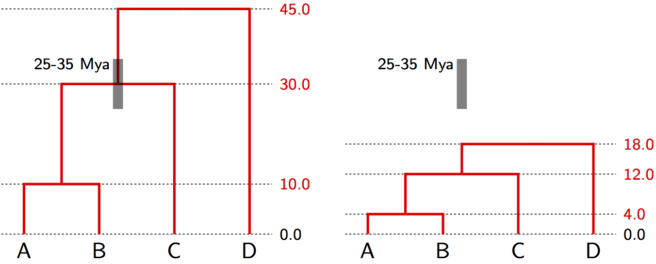
Node Calibration in Practice
- Fossil provides minimum age (fossil must be younger than clade)
- Biogeography can provide maximum age (e.g., island age)
- Often specified as probability distributions (e.g., lognormal)
- Multiple calibrations improve precision
2. Tip Calibrations
Use samples from different time points:
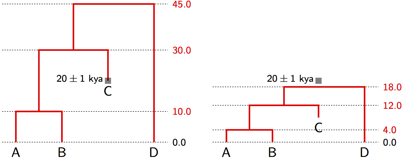
Applications of Tip Calibration
- Ancient DNA: Subfossil remains, museum specimens
- Rapidly evolving pathogens: Virus samples from different years
- Laboratory evolution: Samples from known time points
4. Relaxed Molecular Clocks
The strict molecular clock is often too restrictive. Relaxed clocks allow rate variation across branches.
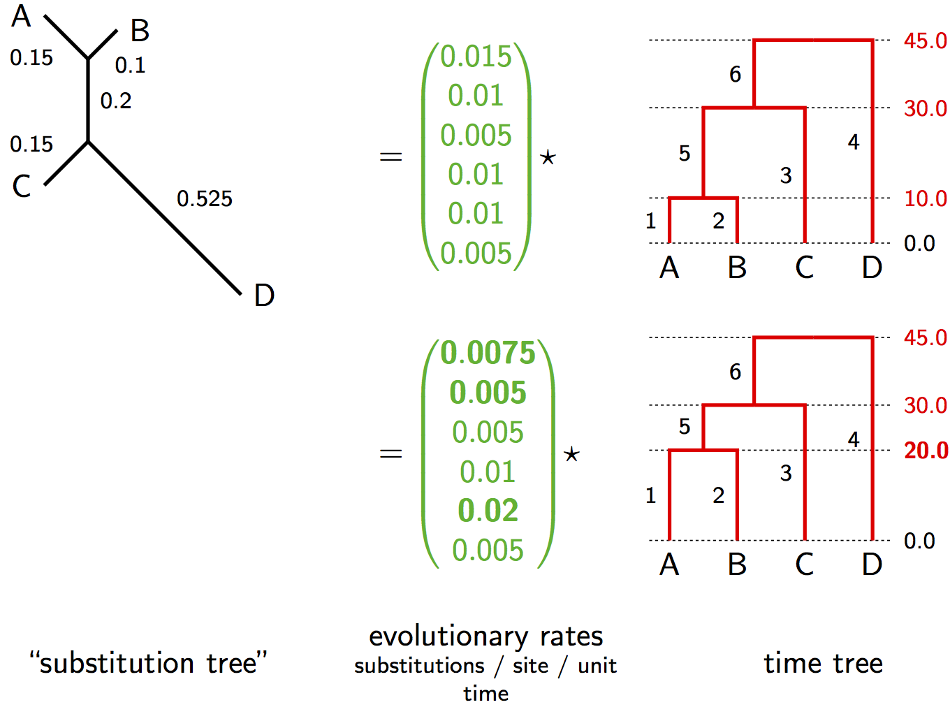
Relaxed Clock Parameterization
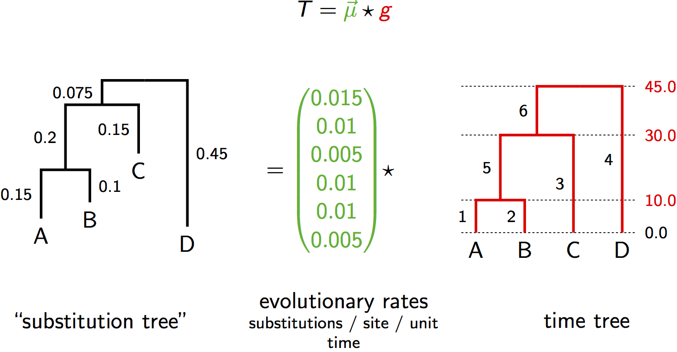
Instead of a single rate $\mu$, we have a vector of rates $\vec{\mu} = (\mu_1, \mu_2, ..., \mu_{2n-2})$
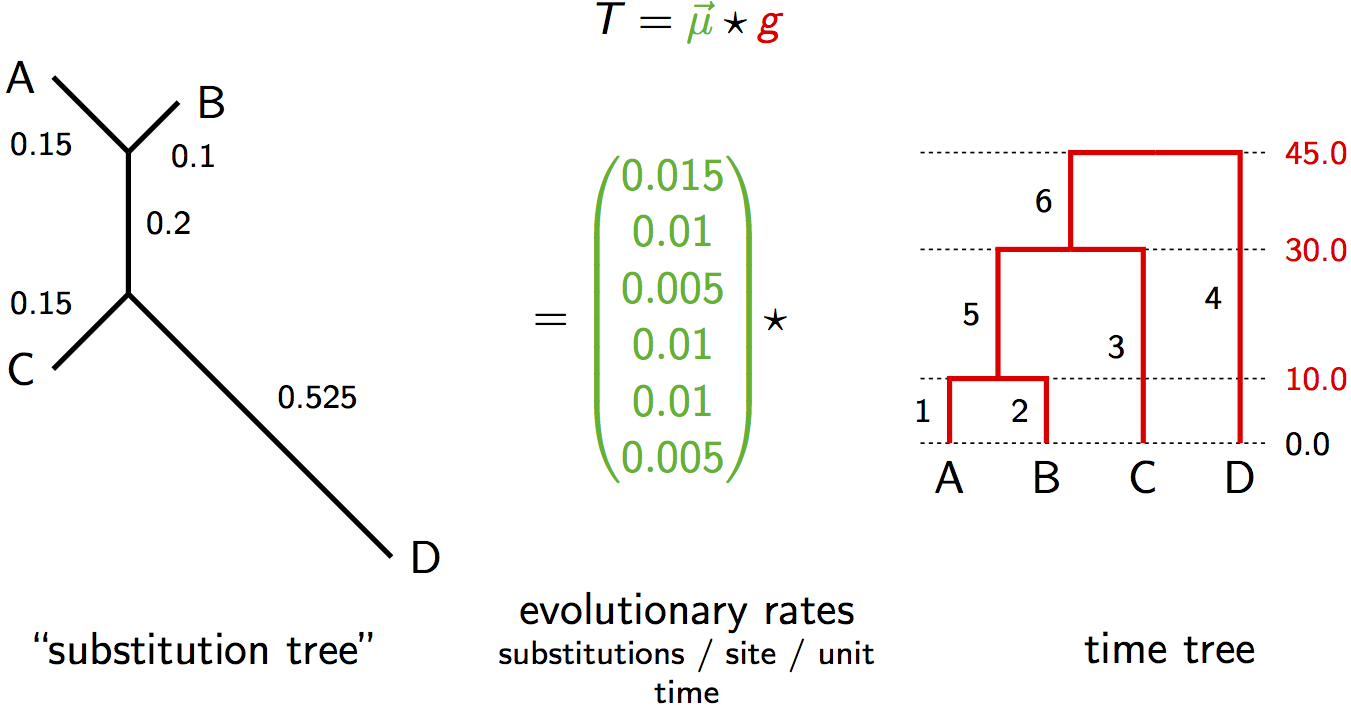
The substitution tree is computed as: $T = \vec{\mu} \star g$
Where $\star$ denotes element-wise multiplication of rates and branch durations
Alternative Relaxed Clock Visualization
Identifiability Under Relaxed Clocks
5. Bayesian Framework for Molecular Clocks
Posterior with Strict Clock
Strict Clock Posterior
Substitution tree: $T = \textcolor{darkgreen}{\mu} \times \textcolor{red}{g}$
Where:
- $\textcolor{red}{g}$ = time tree
- $\textcolor{darkgreen}{\mu}$ = clock rate
- $\theta$ = other model parameters
Posterior with Relaxed Clock
Relaxed Clock Posterior
Substitution tree: $T = \textcolor{darkgreen}{\vec{\mu}} \star \textcolor{red}{g}$
Where $P(\textcolor{darkgreen}{\vec{\mu}})$ is the prior for rate variation
- The phylogenetic likelihood only depends on the substitution tree $T$: $\Pr(D|T)$
- The tree prior only depends on the time tree $\textcolor{red}{g}$: $P(\textcolor{red}{g}|\theta)$
- By fixing $\textcolor{darkgreen}{\vec{\mu}} = 1$, we get a time tree in units of substitutions
6. Models of Rate Variation
Autocorrelated Models
Rates evolve along the tree, with child rates similar to parent rates:
Common implementation: Lognormal autocorrelated model
Where:
- $t_i$ = time duration of branch $i$
- $\sigma$ = rate of evolution of rates (volatility parameter)
Uncorrelated Models
Rates are drawn independently for each branch:
Common implementations:
- Lognormal: $\log(\mu_i) \sim \text{Normal}(M, S)$
- Exponential: $\mu_i \sim \text{Exponential}(\lambda)$
- Gamma: $\mu_i \sim \text{Gamma}(\alpha, \beta)$
Autocorrelated
- Biologically motivated
- Smooth rate changes
- Good for closely related species
- Can extrapolate rates
Uncorrelated
- More flexible
- Allows sudden rate changes
- Good for diverse datasets
- Simpler to implement
7. Parameter Dimensions
Understanding the number of parameters helps us appreciate model complexity:
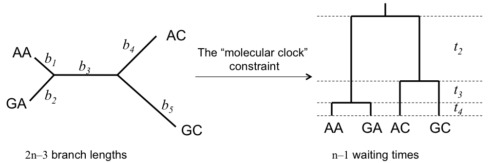
Unrooted Tree (No Clock)
- $2n-3$ branch lengths (one per branch)
- Total: $2n-3$ parameters
Strict Molecular Clock
- $n-1$ node heights (internal nodes)
- 1 clock rate $\mu$
- Total: $n$ parameters
Relaxed Molecular Clock
- $n-1$ node heights
- $2n-2$ rate parameters (one per branch)
- Total: $3n-3$ parameters
8. MCMC Implementation Differences
MrBayes Approach (No Clock)
MrBayes samples unrooted trees without molecular clock constraints:
- Operators must connect any unrooted tree to any other
- Branch lengths can be any positive value
- No temporal constraints
- Simpler operators but no time information
BEAST Approach (With Clock)
BEAST samples rooted time trees with clock constraints:
- Operators must maintain temporal constraints
- All tips fixed at their sampling times
- Internal nodes must be older than descendants
- Natural to work with node heights rather than branch lengths
Clock-Constrained Operators
Examples of operators that maintain temporal constraints:
- Scale: Multiply all node heights by a factor
- Subtree slide: Move subtree up/down while maintaining order
- Wilson-Balding: Prune and regraft with valid node times
- Uniform node height: Sample new height within valid bounds
9. Advantages of Molecular Clock Models
Relaxed molecular clocks offer several benefits over unconstrained models:
- Improved phylogenetic accuracy:
- Rate smoothing helps identify correct topology
- Reduces long-branch attraction artifacts
- Better performance on empirical datasets
- Automatic rooting:
- No need for outgroup
- Root position estimated from rate variation
- Particularly useful when outgroup is distant
- Temporal information:
- Relative divergence times always available
- Absolute times with calibration
- Useful for studying evolutionary rates
- Integration with other models:
- Natural combination with coalescent priors
- Enables epidemiological inference
- Links to fossil data
Summary
This lecture covered two interrelated topics crucial for modern phylogenetics:
- Tree space geometry:
- Trees exist in a complex space with discrete and continuous components
- Each topology defines a subspace of dimension $n-1$
- Understanding tree space helps design better algorithms
- Molecular clocks:
- Fundamental equation: distance = rate × time
- Rate and time are non-identifiable without calibration
- Strict clocks assume constant rates
- Relaxed clocks allow rate variation
- Bayesian implementation:
- Priors essential for identifiability
- Different parameterizations for different software
- MCMC must respect temporal constraints
- Practical advantages:
- Better tree estimation
- Automatic rooting
- Temporal information
- Integration with other evolutionary models
- Drummond & Bouckaert (2015) "Bayesian Evolutionary Analysis with BEAST" - Chapters 6-7
- Yang (2014) "Molecular Evolution: A Statistical Approach" - Chapter 7
- Drummond et al. (2006) "Relaxed phylogenetics and dating with confidence" - PLOS Biology
- Billera et al. (2001) "Geometry of the space of phylogenetic trees" - Advances in Applied Mathematics
Check Your Understanding
- Why is tree space not a simple Euclidean space?
- What makes rate and time non-identifiable in molecular evolution?
- How do node and tip calibrations solve the identifiability problem?
- What's the key difference between autocorrelated and uncorrelated relaxed clocks?
- Why do relaxed clocks often produce better phylogenetic estimates than no-clock models?