Likelihood and Substitution Models - Bayesian phylogenetics lectures

1. Problems with Parsimony

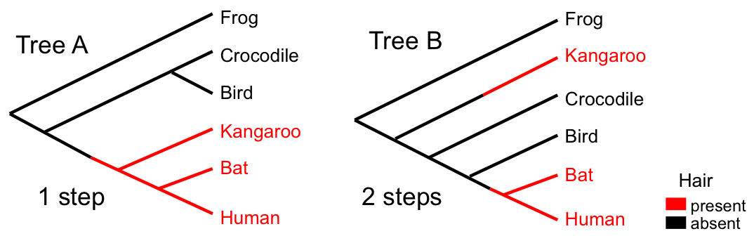
Recall: parsimony seeks trees with minimum number of changes

While parsimony is intuitive and computationally tractable for small problems, it has several limitations:

"Large parsimony problem" is computationally expensive
- NP-hard problem requiring heuristic search algorithms
- No guarantee of finding global optimum
Gives point estimates with no uncertainty quantification
- No confidence intervals or support values
- No way to compare alternative hypotheses statistically
Questionable biological basis
- Assumes all changes are equally unlikely
- Ignores branch lengths
Not model-based
- No formal hypothesis testing
- No model comparison
Hidden problems
- Long branch attraction
- Inconsistency under certain conditions

Key insight: We need a model-based approach that can quantify uncertainty and allow formal hypothesis testing.

2. Modelling Neutral Sequence Evolution

Why Use Models?

We need a model to relate what we observe (data) to what we want to know (hypotheses and parameters).

Fundamental principle: Inference is not possible without a model!

We use probabilistic models for molecular evolution because:

We don't know enough about mutation mechanisms for deterministic models
Stochastic effects are important at molecular level
Allows uncertainty quantification
Enables formal statistical inference

Genetic Distance: From p-distance to Model-based Estimates

The p-distance

p-distance

The proportion of sites that differ between two aligned sequences.

Example: If 15 out of 100 sites differ, p-distance = 0.15

Simple to calculate
Always between 0 and 1
Also called normalized Hamming distance
BUT: underestimates true evolutionary distance (we'll see why)

Computing p-distance between aligned sequences

p-distance Example

p-distance = 3/7 ≈ 0.43

Interpretation: 43% of sites differ between these sequences

Why p-distance Underestimates True Distance

The p-distance usually underestimates the true genetic (evolutionary) distance because it doesn't account for:

Multiple, parallel, and back-substitutions are invisible in pairwise comparisons

Biological Intuition

Imagine watching a bird feeder at different times:

You see a korimako/bellbird at 9am and you again see a korimako/bellbird at 5pm.
Same bird all day? Or did multiple birds use the spot?
Without continuous observation, you can't tell!

Similarly, DNA sites may have changed multiple times between ancestors and descendants.

Multiple substitutions: Same site changing more than once
Parallel substitutions: Same change occurring independently
Back-substitutions: Reversions to ancestral state

Relationship Between p-distance and Genetic Distance

The p-distance saturates at 0.75 for random sequences, while true genetic distance continues to increase

Why does p-distance saturate at 0.75?

With 4 nucleotides and random substitutions:

Probability of staying the same = 1/4
Probability of being different = 3/4
After infinite time, sequences become random with respect to each other
Random sequences differ at 75% of sites

3. Continuous-Time Markov Chains (CTMCs)

Mathematical Framework

Continuous-Time Markov Chain

A stochastic process where:

State X(t) is a function of continuous time
Future states depend only on current state (Markov property)
Transition rates are constant over time

What does this mean biologically?

A continuous-time Markov chain models how nucleotides change over time:

Each site evolves independently
Changes can happen at any time
The probability of change depends only on current state, not history
Like radioactive decay - constant probability of change per unit time

Example: An 'A' nucleotide doesn't "remember" how long it's been an 'A' - it always has the same probability of mutating in the next instant.

CTMCs obey the Chapman-Kolmogorov equation:

P(X(t_1)|X(t_0)) = \sum_{X(t_i)} P(X(t_1)|X(t_i))P(X(t_i)|X(t_0))

In plain English: To get from state X(t₀) to X(t₁), sum over all possible paths through intermediate states.

Mathematical Details (Optional)

This section provides mathematical depth for those interested. Biology-focused readers can skip to the next section.

The differential form (Master equation/Kolmogorov forward equation):

\frac{d}{dt}p(x,t|x_0,t_0) = \sum_{x'} Q_{x'x}p(x',t|x_0,t_0)

Where Q is the instantaneous rate matrix with:

\(Q_{ij}\) = rate of change from state i to j (i ≠ j)
\(Q_{ii} = -\sum_{j \neq i} Q_{ij}\) (rows sum to zero)

Relationship Between Q and P(t)

Key Relationship

The transition probability matrix P(t) is the matrix exponential of Qt:

P(t) = \exp(Qt) = \sum_{k=0}^{\infty} \frac{(Qt)^k}{k!} = I + tQ + \frac{(tQ)^2}{2!} + \frac{(tQ)^3}{3!} + \ldots

Intuition for the Matrix Exponential

This formula tells us:

P(0) = I (no time = no change)
P(small t) ≈ I + tQ (short time = approximately linear)
P(large t) → stationary distribution (long time = equilibrium)

Think of it as compound interest for mutations!

CTMC Example

Two-State System

Consider a simplified DNA with only purines (R) and pyrimidines (Y):

Q = \begin{bmatrix} -2 & 2 \\ 1 & -1 \end{bmatrix}

This means:

Rate R→Y: 2 per unit time
Rate Y→R: 1 per unit time

Biological interpretation: Transitions (R↔Y) happen at different rates in each direction

Time spent in state before transition follows exponential distribution:

P(\Delta t|x) = \lambda e^{-\lambda \Delta t}

where \(\lambda = -Q_{xx}\) is the total rate of leaving state x.

Time-Reversibility and Detailed Balance

Time-Reversible CTMC

A CTMC is time-reversible if it satisfies detailed balance:

\pi_i Q_{ij} = \pi_j Q_{ji}

where π is the stationary distribution.

For time-reversible CTMCs:

Process looks the same forward and backward in time
Stationary distribution satisfies: \(\pi Q = 0\)
Mathematical convenience for phylogenetics
Important: No biological justification required!

Note: We assume time-reversibility for mathematical convenience, not because evolution looks the same in both directions!

4. DNA Substitution Models

Now let's see how CTMCs are used to model DNA evolution. We'll start simple and build complexity.

Jukes-Cantor (JC69) Model

The Simplest Model

Assumptions:

All substitutions equally likely
Equal base frequencies (25% each)
One parameter: μ (overall rate)

Rate matrix:

Q = \mu \begin{bmatrix} -1 & \frac{1}{3} & \frac{1}{3} & \frac{1}{3} \\ \frac{1}{3} & -1 & \frac{1}{3} & \frac{1}{3} \\ \frac{1}{3} & \frac{1}{3} & -1 & \frac{1}{3} \\ \frac{1}{3} & \frac{1}{3} & \frac{1}{3} & -1 \end{bmatrix}

Transition probabilities:

P_{ij}(t) = \begin{cases} \frac{1}{4} + \frac{3}{4}e^{-\frac{4}{3}\mu t} & \text{if } i = j \text{ (same nucleotide)} \\ \frac{1}{4} - \frac{1}{4}e^{-\frac{4}{3}\mu t} & \text{if } i \neq j \text{ (different nucleotide)} \end{cases}

Genetic Distance Under JC69

Given observed p-distance, we can estimate the true genetic distance:

\hat{d} = -\frac{3}{4}\log\left(1 - \frac{4}{3}p\right)

Limitations:

Formula undefined if p ≥ 3/4 (sequences too divergent)
Assumes all changes equally likely (unrealistic)
Assumes equal base composition (often violated)

Kimura 2-Parameter (K80) Model

Adding Biological Realism

Key innovation: Transitions ≠ Transversions

Transitions (α): Purine↔Purine, Pyrimidine↔Pyrimidine
Transversions (β): Purine↔Pyrimidine
Usually α > β (transitions more common)

Rate matrix:

Q = \begin{bmatrix} \cdot & \alpha & \beta & \beta \\ \alpha & \cdot & \beta & \beta \\ \beta & \beta & \cdot & \alpha \\ \beta & \beta & \alpha & \cdot \end{bmatrix}

Why are transitions more common?

Chemical similarity:

Purines (A,G): Two-ring structures
Pyrimidines (C,T): One-ring structures
Replacing like-with-like causes less structural disruption

HKY Model

Hasegawa-Kishino-Yano (1985)

Features:

Different transition/transversion rates
Unequal base frequencies (πA, πC, πG, πT)
Reflects GC-content variation

Rate matrix:

Q = \begin{bmatrix} \cdot & \alpha\pi_C & \beta\pi_G & \beta\pi_T \\ \alpha\pi_A & \cdot & \beta\pi_G & \beta\pi_T \\ \beta\pi_A & \beta\pi_C & \cdot & \alpha\pi_T \\ \beta\pi_A & \beta\pi_C & \alpha\pi_G & \cdot \end{bmatrix}

General Time Reversible (GTR) Model

The Most General Model

Features:

All substitution types can have different rates
6 rate parameters + 4 frequency parameters
Most flexible time-reversible model
Includes all previous models as special cases

Rate matrix:

Q = \begin{bmatrix} \cdot & \alpha\pi_C & \beta\pi_G & \gamma\pi_T \\ \alpha\pi_A & \cdot & \delta\pi_G & \epsilon\pi_T \\ \beta\pi_A & \delta\pi_C & \cdot & \eta\pi_T \\ \gamma\pi_A & \epsilon\pi_C & \eta\pi_G & \cdot \end{bmatrix}

Model Comparison Summary

Model	Parameters	Key Feature	When to Use
JC69	1	All equal	Very similar sequences
K80	2	Ts/Tv ratio	Moderate divergence
HKY	5	+Base frequencies	GC-content varies
GTR	9	All different	Complex datasets

Rate Heterogeneity Among Sites

Biological Reality

Not all sites in a gene evolve at the same rate:

Active sites: Highly conserved (slow evolution)
Structural regions: Moderate constraints
Surface loops: Fewer constraints (fast evolution)
Synonymous sites: Often evolve fastest

We model rate variation using a gamma distribution:

f(r) = \frac{\alpha^\alpha}{\Gamma(\alpha)} r^{\alpha-1} e^{-\alpha r}

Different values of α give different rate distributions. Small α = high variation

Understanding the shape parameter α

α < 1: Most sites evolve slowly, few evolve very fast
α = 1: Exponential distribution
α > 1: Bell-shaped distribution
α → ∞: All sites evolve at same rate

Model Comparison Example

HIV Distance Estimates

HIV-1B vs other strains (env gene):

Comparison	p-distance	JC69	K80	Tajima-Nei
HIV-O	0.391	0.552	0.560	0.572
SIVcpz	0.266	0.337	0.340	0.427
HIV-1C	0.163	0.184	0.187	0.189

Observation: Model choice matters more for divergent sequences!

5. Likelihood-Based Phylogenetic Inference

From Distances to Likelihood

Distance methods lose information by summarizing sequences as pairwise distances. Likelihood methods use all the data.

The Likelihood Function

Likelihood

The likelihood for parameter θ under model M given data D is:

L(\theta|D,M) \equiv P(D|\theta,M)

In words: "The probability of observing our data if the parameter values were θ"

Important: The likelihood is NOT a probability distribution over θ!

Simple Example: Coin Flips

5 tosses give: D = (H,T,T,H,T)

What's the probability of getting exactly this sequence?

P(D|f) = f \times (1-f) \times (1-f) \times f \times (1-f) = f^2(1-f)^3

This is the likelihood function L(f|D)!

The likelihood peaks at f = 2/5 = 0.4 (we observed 2 heads in 5 flips)

Maximum Likelihood Inference

The maximum likelihood estimate is the parameter value that makes the observed data most probable.

Why Maximum Likelihood?

Intuitive: Choose parameters that make data most likely
Optimal properties: Consistent, efficient (with enough data)
General framework: Works for any statistical model
BUT: Only gives point estimates, no uncertainty!

Tree Likelihood

For phylogenetics, we want P(alignment | tree, model):

Computing likelihood requires summing over all possible ancestral states

The likelihood calculation involves:

For each site in the alignment:
- Consider all possible ancestral states
- Calculate probability of observing tip states
- Sum over all possibilities
Multiply across sites (assumes independence)

Computational challenge: For n taxa with DNA, there are 4^(n-1) possible combinations of internal node states per site!

Felsenstein's Pruning Algorithm

Joseph Felsenstein (1973) solved this using dynamic programming:

The Pruning Algorithm

Key idea: Work from tips toward root, storing partial likelihoods

Define: L_k(s) = likelihood of subtree below node k if node k has state s

For leaf nodes:

L_k(s) = \begin{cases} 1 & \text{if leaf has state } s \\ 0 & \text{otherwise} \end{cases}

For internal nodes with children i and j:

L_k(s) = \left(\sum_x P(x|s,t_i)L_i(x)\right)\left(\sum_y P(y|s,t_j)L_j(y)\right)

Where P(x|s,t) is the probability of state s changing to x in time t

Why This Works

Instead of considering all 4^(n-1) combinations:

Store 4 numbers at each node (partial likelihoods)
Build up from tips to root
Reuse calculations (dynamic programming principle)

Result: Linear time in number of taxa!

Maximum Likelihood Software

ML Phylogenetic Software

IQ-TREE (Nguyen et al., 2015)
- State-of-the-art tree search
- Automatic model selection
- Ultrafast bootstrap
RAxML (Stamatakis, 2014)
- Highly optimized for large datasets
- Excellent parallelization
- Standard in many pipelines
PhyML (Guindon et al., 2010)
- User-friendly
- Good for moderate datasets
- Fast approximate likelihood ratio tests
FastTree (Price et al., 2009)
- Approximate but very fast
- Can handle millions of sequences
- Good for initial analyses

Limitations of Maximum Likelihood

ML gives us a point estimate with no measure of uncertainty!

No confidence intervals
- How certain are we about the tree?
- Bootstrap provides some help (but it's ad hoc)
Model selection challenges
- How do we choose between JC69, K80, HKY, GTR?
- Likelihood ratio tests only work for nested models
Can't incorporate prior knowledge
- What if we know some clades are unlikely?
- What if we have fossil calibrations?

We need a framework that handles uncertainty properly → Bayesian inference!

Summary

This lecture introduced model-based phylogenetic inference:

Why models?
- Parsimony has serious limitations
- Models enable statistical inference
- Can test hypotheses formally
Substitution models as CTMCs:
- Continuous-time Markov chains model sequence evolution
- Models range from simple (JC69) to complex (GTR+Γ)
- More complex models fit data better but risk overfitting
Key biological insights:
- p-distance underestimates true distance due to multiple hits
- Transitions more common than transversions
- Base composition varies across genomes
- Different sites evolve at different rates
Likelihood methods:
- Use all information in the alignment
- Felsenstein's algorithm makes computation feasible
- BUT: still only point estimates
Next step: Bayesian inference provides a complete framework for uncertainty

Key Takeaways

For biologists: Models let us correct for unseen changes and test evolutionary hypotheses
For computer scientists: Phylogenetics offers rich algorithmic challenges (DP, matrix exponentials, tree search)
For everyone: Understanding models is crucial for interpreting phylogenetic results

Recommended Reading:

Felsenstein (2004) "Inferring Phylogenies" - Chapters 13-16
Yang (2014) "Molecular Evolution: A Statistical Approach" - Chapters 1-2
Drummond & Bouckaert (2015) "Bayesian Evolutionary Analysis with BEAST" - Chapter 2

Check Your Understanding

Why does p-distance underestimate true evolutionary distance?
What biological reasons explain why transitions are more common than transversions?
How does Felsenstein's algorithm achieve computational efficiency?
What are the key differences between JC69, K80, HKY, and GTR models?
Why isn't likelihood a probability distribution over parameters?