MCMC in Phylogenetics
1. The Phylogenetic Likelihood
At the heart of Bayesian phylogenetic inference is the phylogenetic likelihood:
Where:
- $D$ is a multiple sequence alignment of $n$ sequences
- $T$ is a phylogenetic tree with $n$ leaves
- $\mu$ are the parameters of the chosen CTMC-based model of sequence evolution
Computing the Likelihood
The phylogenetic likelihood is computed using Felsenstein's pruning algorithm (covered in Lecture 7). Key points:
- The likelihood is a product of site pattern probabilities
- Sites are assumed to evolve independently
- This assumption allows for obvious generalizations:
- Multiple alignments that share a tree
- Phylogenetic networks where different sites evolve under distinct "local" trees
2. The Phylogenetic Posterior
Standard application of Bayes' theorem gives the posterior:
Factorizing the Posterior
Most phylogenetic models make two key assumptions:
- $\theta$ only affects the probability of the data via the tree $T$
- $\mu$ has no effect on the tree branching process
These assumptions lead to the factorized form:
Phylogenetic Posterior
Where:
- $P(T|\theta)$ is the "tree prior" parameterized by $\theta$
- $P(\mu,\theta)$ are the parameter priors
- $P(D)$ is the marginal likelihood (evidence)
Questions to Consider
- What is $P(D)$ and why is it difficult to compute?
- Is the tree prior really a prior? (i.e., does it depend on the data?)
The Neutrality Assumption
The factorization above implicitly assumes that our alignment could have been produced through the following process:

3. Tree Priors
Tree priors allow us to specify a generative model for the genealogy. While this model may not involve genetic evolution, it may depend on:
- Speciation rates
- Population sizes
- Migration rates
- Extinction rates
- Sampling processes
The Yule Model for Speciation
The simplest tree prior is the Yule model (Yule, 1924):
- Constant rate branching process
- Branching occurs uniformly across extant lineages at rate $\lambda$ per lineage per unit time
- Chemical kinetics formalism: $X \overset{\lambda}{\longrightarrow} 2X$
The number of lineages $k$ evolves under the master equation:

Birth-Death(-Sampling) Priors
A more realistic model accounts for both speciation and extinction:
- Generalization of Yule process to account for extinction and sampling
- Linear speciation, extinction, and sampling rates
- Prior is over sampled trees: assumes unobserved full tree
- Groundwork largely due to Tanja Stadler (ETH Zürich)

Coalescent Priors
For modeling gene trees within populations:
- Original theory due to Kingman (1980)
- Models the shape of gene trees within a species
- Can be obtained as the limit of population genetic models (Wright-Fisher, Moran)
- Provides crucial link between tree shape and population size

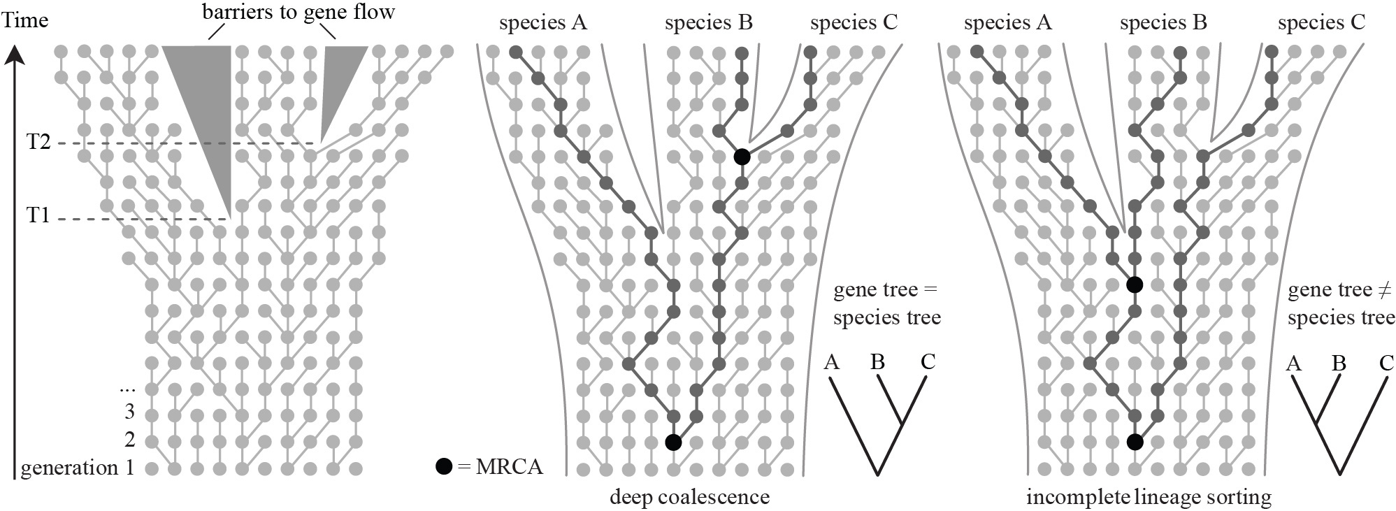
Multi-species Coalescent Priors
Hierarchical models that embed gene trees within species trees:
- Species tree described using a birth-death prior
- Gene trees described by coalescent priors for populations which subdivide at speciation events
- Accounts for incomplete lineage sorting
4. MCMC in Tree Space
Basic MCMC Theory Review
MCMC works by simulating a stochastic trajectory according to:
Where the transition kernel is:
Detailed Balance and Acceptance Probability
A sufficient condition for $\pi(x)$ to be the equilibrium distribution is detailed balance:
This is satisfied by the Metropolis-Hastings acceptance probability:
Metropolis-Hastings Acceptance
Key Properties for Tree Space
- By tuning the acceptance probability, any probability distribution can be targeted
- Only the ratio $\pi(x')/\pi(x)$ appears: normalization need not be known
- The only requirement for $q(x'|x)$ is irreducibility: random walks must explore the entire state space
- For high-dimensional state spaces, $W(x'|x)$ is decomposed into several distinct operators: $W(x'|x)=\sum_j W_j(x'|x)$
- The ratio $q(x|x')/q(x'|x)$ is the Hastings ratio
5. Proposal Distributions for Trees
We need to identify a set of proposals $q_j(x'|x)$ when $x$ is a point in the space of rooted time trees.

Common Tree Operators
- Subtree Slide
- Move a subtree up or down along a branch, changing node heights
- Wilson-Balding
- Prune a subtree and regraft it elsewhere, sampling new node times
- Narrow/Wide Exchange
- Swap two subtrees that share a grandparent (narrow) or any two subtrees (wide)
- Node Height Changes
- Modify the height of internal nodes while maintaining time consistency
- Tree Scaling
- Scale all node heights by a common factor
Hastings Ratios for Tree Operators
Computing the Hastings ratio for tree operators can be complex:
- Must account for changes in the number of possible attachment points
- Node height proposals may have different forward/reverse probabilities
- Some operators (e.g., uniform tree scaling) have trivial Hastings ratios
Example: Subtree Slide Hastings Ratio
For a subtree slide that moves node $v$ from time $t$ to $t'$:
- If heights are proposed uniformly in valid ranges
- Forward range: $(t_{\text{child}}, t_{\text{parent}})$
- Reverse range: $(t'_{\text{child}}, t'_{\text{parent}})$
- Hastings ratio: $\frac{t'_{\text{parent}} - t'_{\text{child}}}{t_{\text{parent}} - t_{\text{child}}}$
6. Convergence and Mixing
Stopping Criteria
Two critical questions for phylogenetic MCMC:
- How can we tell when the chain has reached equilibrium?
- How do we know when we've collected enough samples?
Effective Sample Size (ESS)
One approach is to compute ESS for each parameter and tree summary statistics:
- ESS estimates the number of independent samples
- Common statistics to monitor:
- Tree height (age of root)
- Tree length (sum of branch lengths)
- Model parameters (substitution rates, etc.)
- Rule of thumb: ESS > 200 for all parameters
Multiple Independent Runs
Assessing Tree Convergence
Trees present special challenges for convergence assessment:
- Cannot plot simple traces of "the tree"
- Need specialized statistics for tree space
- Common approaches:
- Compare split frequencies between runs
- Average standard deviation of split frequencies (ASDSF)
- Tree distance metrics between samples
AWTY (Are We There Yet?)
Software that applies multiple statistics to assess tree convergence:
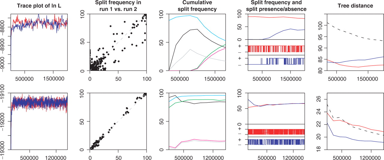
Key diagnostics:
- Split frequency correlations between runs
- Cumulative split frequencies over time
- Tree space visualization using multidimensional scaling
7. Post-processing MCMC Output
Parameter Samples
Logs of individual parameters can be considered samples from marginal posteriors:
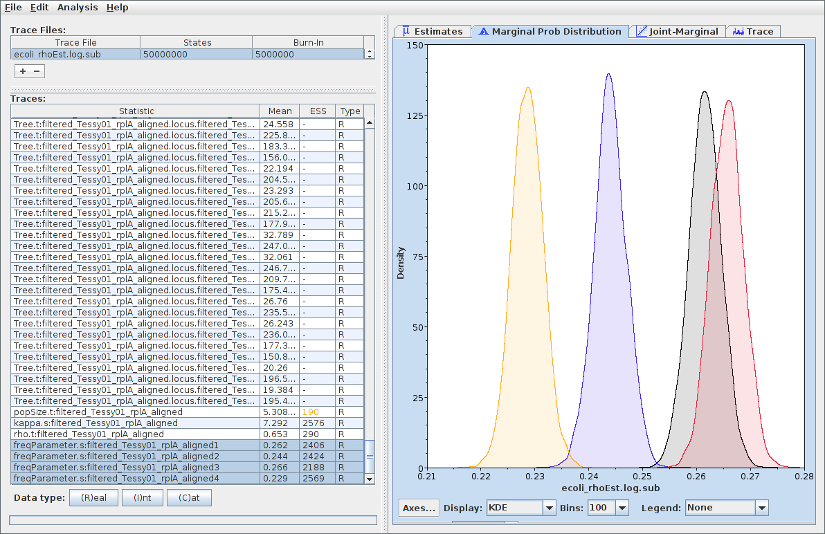
Common analyses:
- Marginal density estimation
- 95% credible intervals
- Mean/median estimates
- Correlation between parameters
Tree Samples
Summary Statistics
Extract specific information from sampled trees:
- Age of MRCA for clades of interest
- Posterior probabilities of clades
- Branch length distributions
- Tree balance statistics
Summary Trees
Different approaches to produce a single "summary" tree:
- Strict Consensus
- Include only clades that appear in ALL sampled trees
- Majority Rule Consensus
- Include clades that appear in >50% of sampled trees
- Maximum Clade Credibility (MCC) Tree
- The sampled topology for which the product of posterior clade probabilities is maximized
8. Bayesian Phylogenetic Software
General Purpose Software
- MrBayes (Huelsenbeck and Ronquist, 2001)
-
- Early command-line program for phylogenetic inference
- Implements standard substitution models and tree priors
- Widely used and well-tested
- RevBayes (Höhna et al., 2016)
-
- R-like syntax for specifying phylogenetic models
- Highly flexible model specification
- Growing ecosystem of tutorials and methods
- BEAST/BEAST 2 (Drummond and Rambaut, 2007; Bouckaert et al., 2014)
-
- XML specification of phylogenetic models
- Extensible through packages
- Strong focus on time-calibrated trees
- Integrated with other tools (BEAUti, Tracer, TreeAnnotator)
Specialized Software
- MIGRATE
- Performs inference under the Structured Coalescent (subpopulation sizes, migration rates, ancestral locations)
- ClonalFrame/ClonalOrigin
- Infer bacterial Ancestral Recombination Graphs (generalizations of trees when recombination is present)
Software Ecosystem
- BEAUti: GUI for creating BEAST XML files
- Tracer: MCMC trace analysis and diagnostics
- FigTree: Tree visualization and annotation
- DensiTree: Visualizing sets of trees
- SPREAD: Spatial phylogenetic reconstruction
Summary
This lecture covered the practical aspects of Bayesian phylogenetic inference using MCMC:
- Phylogenetic posterior: Combines tree likelihood with tree priors under neutrality assumption
- Tree priors:
- Yule process (pure birth)
- Birth-death-sampling models
- Coalescent and multi-species coalescent
- MCMC in tree space:
- Requires specialized operators
- Must maintain time consistency
- Complex Hastings ratios
- Convergence assessment:
- ESS for parameters and tree statistics
- Multiple independent runs essential
- Specialized diagnostics for trees
- Post-processing:
- Parameter estimation straightforward
- Tree summarization challenging
- Report uncertainty, not just point estimates
- Tree priors link tree shape to biological processes
- MCMC makes Bayesian phylogenetics computationally feasible
- Convergence assessment is crucial but challenging
- No single summary can capture complex posteriors
- Felsenstein (2004) "Inferring Phylogenies" - Chapters 26-27
- Drummond & Bouckaert (2015) "Bayesian Evolutionary Analysis with BEAST" - Chapters 4-5
- Yang (2014) "Molecular Evolution: A Statistical Approach" - Chapter 7
- Höhna et al. (2016) "RevBayes: Bayesian phylogenetic inference" - Systematic Biology
Check Your Understanding
- Why does the phylogenetic posterior factorization imply neutral evolution?
- What's the difference between birth-death and coalescent tree priors?
- Why do we need specialized operators for tree space MCMC?
- What makes ESS a useful but imperfect convergence diagnostic?
- Why might an MCC tree be misleading for multimodal posteriors?