Bayesian Inference
1. Probability as Extended Logic
From Logic to Plausible Reasoning
Traditional deductive logic is based on syllogisms that provide certain conclusions:
If A is true, then B is true
A is true
Therefore, B is true
If A is true, then B is true
B is false
Therefore, A is false
But real-world reasoning often requires handling uncertainty. Consider this scenario:
Suppose some dark night a policeman walks down a street. He hears a burglar alarm, looks across the street, and sees a jewelry store with a broken window. Then a gentleman wearing a mask comes crawling out of the window, carrying a bag full of jewelry. The policeman decides immediately that the gentleman is a thief. How does he decide this? — E.T. Jaynes, Probability Theory
Let's analyze this:
- A: "the gentleman is a thief"
- B: "the gentleman is wearing a mask and exited a broken window holding a bag of jewelry"
The policeman appears to use a weak syllogism:
If A is true, then B is likely
B is true
Therefore, A is likely
Developing a Theory of Plausible Reasoning
To formalize reasoning under uncertainty, our theory must satisfy:
- Degrees of plausibility are represented by real numbers
- Qualitative correspondence with common sense
- Consistency:
- All valid reasoning routes give the same result
- Equivalent states of knowledge have equivalent plausibilities
These requirements uniquely identify the rules of probability theory!
- Richard Cox (1946) showed that any consistent system for plausible reasoning must follow the rules of probability
- Probability theory is thus the unique extension of logic to handle uncertainty
The Rules of Probability
From Cox's axioms, we derive:
Fundamental Rules
- Probability: $P(A|B)$ is the degree of plausibility of proposition A given that B is true
- Product Rule: $P(A,B|C) = P(A|B,C)P(B|C)$
- Sum Rule: $P(A|B) + P(\neg A|B) = 1$
By convention: $P(A) = 0$ means A is certainly false; $P(A) = 1$ means A is certainly true
Notation and Continuous Variables
For continuous variables, we use probability densities:
- If X can take any value between 0 and 10, then $P(X = x) = 0$ always
- Instead, define: $P(x < X < x + \delta) = \delta f(x)$
- $f(x)$ is a probability density
- Normalization: $\int_0^{10} f(x)dx = 1$
- Non-negative: $f(x) \geq 0$
- Can have $f(x) > 1$ at specific points!
Bayesian vs. Frequentist Interpretations
Frequentist
- Probability = long-run frequency
- Requires repeatable experiments
- Assumes randomness is inherent
- Cannot assign probabilities to hypotheses
Bayesian
- Probability = degree of belief
- Works for unique events
- Uncertainty due to incomplete information
- Can reason about any proposition
Example illustrating the difference:

Justifications for the Bayesian Approach
- Axiomatic approach
- Derivation from axioms for manipulating reasonable expectations (Cox's theorem)
- Dutch book approach
- If probability rules aren't followed for gambling odds, one party can always win
- Decision theory approach
- Every admissible statistical procedure is either Bayesian or a limit of Bayesian procedures
2. Bayesian Inference
What is Inference?
The act of deriving logical conclusions from premises when the premises are not sufficient to draw conclusions without uncertainty.
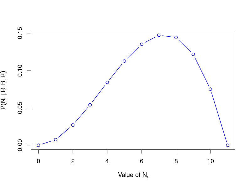
Example: The Urn Problem
Setup

- An urn contains 11 balls: $N_r$ red and $11 - N_r$ blue
- We draw a ball, record its color, and replace it
- Repeat 3 times, obtaining: R, B, R
Question: What is $P(N_r | d_1=R, d_2=B, d_3=R)$?
Solution
First, calculate the likelihood:
Apply the product rule to get:
Where:
- $P(R,B,R | N_r)$ is the likelihood
- $P(N_r)$ is the prior probability
- $P(R,B,R)$ is a normalization constant
Bayes' Theorem
The urn example illustrates the general form of Bayes' theorem:
Bayes' Theorem
Where:
- Posterior $P(\theta_M|D,M)$: Updated belief about parameters after seeing data
- Likelihood $P(D|\theta_M,M)$: Probability of data given parameters
- Prior $P(\theta_M|M)$: Initial belief about parameters
- Evidence $P(D|M)$: Marginal likelihood, normalizing constant
3. Prior Probabilities
What is a Prior?
A prior is simply a probability — specifically, the probability of your hypothesis in the absence of the specific data you're about to analyze.
Key points about priors:
- In principle, two rational people with the same information should specify the same prior
- In practice, this often doesn't happen due to different background knowledge
- Priors are necessary — you cannot do inference without assumptions
- Frequentist methods also use priors implicitly
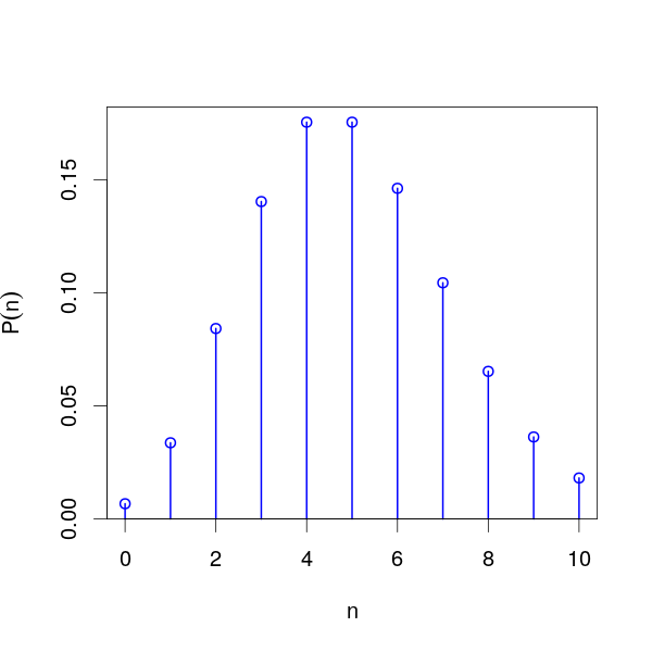
Priors for Discrete Variables
- Finite support: Often use uniform distribution (principle of indifference)
- Count data: Poisson distribution may be appropriate
- Maximum entropy: Choose the distribution with maximum entropy subject to constraints
Priors for Continuous Variables
For bounded continuous variables $a < x < b$:
- Uniform: $f(x) = 1/(b-a)$
- Beta: $f(x) \propto (x-a)^{\alpha-1}(b-x)^{\beta-1}$
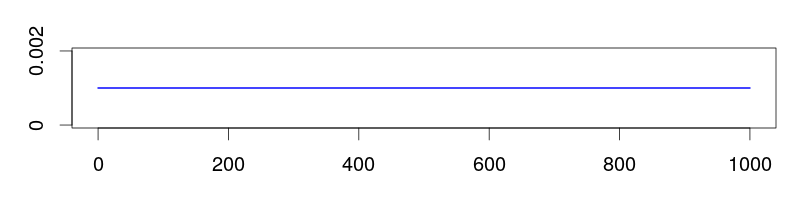
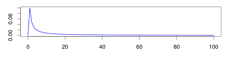
For positive rate parameters $\lambda > 0$:
- Uniform: $f(\lambda) = c$ (improper!)
- Jeffreys: $f(\lambda) = 1/\lambda$ (uniform in log space)
- Log-normal: Proper alternative to Jeffreys prior
Improper Priors
Remember:
- One almost never knows absolutely nothing
- Upper and lower bounds can almost always be placed
- Log-normal can replace the improper $1/x$ prior
Which Prior is Best?
Only the person doing the analysis can answer this! Priors encapsulate expert knowledge (or its absence). This is your opportunity to contribute your expertise to the analysis.
4. Summarizing Uncertainty
Credible Intervals
Bayesian credible intervals summarize uncertainty in parameter estimates:
Credible Interval (Bayesian)
- Given the data, 95% probability the parameter is in this interval
- Direct probability statement
- Depends on prior
Confidence Interval (Frequentist)
- 95% of such intervals contain the true value
- No probability statement about this specific interval
- Prior-free (supposedly)
5. Inference in Practice
The Computational Challenge
Bayes' theorem has a troublesome denominator:
The evidence $P(D|M)$ requires integration:
- Rarely can this integral be solved analytically
- For high-dimensional $\theta_M$, numerical integration is infeasible
Monte Carlo Methods
Algorithms that produce random samples to characterize probability distributions.

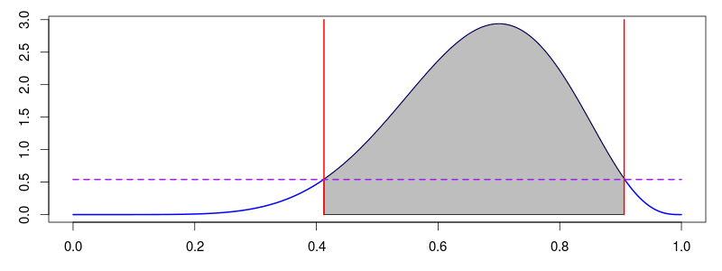
Rejection Sampling
One of the simplest Monte Carlo methods:
Rejection Sampling Algorithm
- Find an envelope distribution that bounds the target
- Sample uniformly under the envelope
- Accept samples under the target distribution
- Reject samples above the target

The Curse of Dimensionality

As dimensions increase, the fraction of the envelope occupied by the target diminishes rapidly. For high-dimensional problems, rejection sampling becomes impractical.
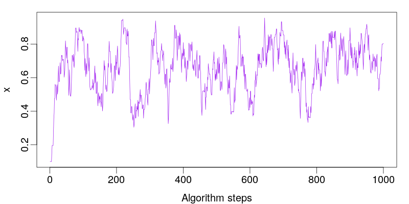
Markov Chain Monte Carlo (MCMC)
The Metropolis-Hastings algorithm generates samples by creating a random walk:

Key advantages:
- Walk explores mostly high-probability areas
- Does not require normalized target distribution
- Works in high dimensions
MCMC Output
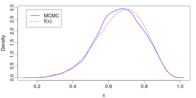
Convergence and Mixing
MCMC challenges:
- Adjacent samples are correlated
- Initial state is arbitrary (burn-in needed)
- Must assess convergence and mixing

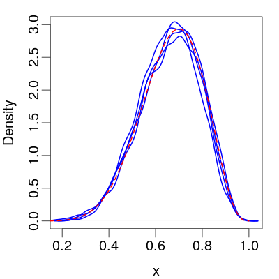
Assessing Convergence
Compare multiple chains from different starting points:
Assessing Mixing
Use the autocorrelation function:
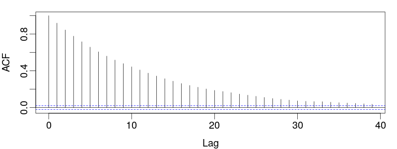
Where N is total samples and τ is the autocorrelation time. ESS estimates the number of independent samples.
Other Approaches
- Monte Carlo Methods
-
- Gibbs sampling
- Hamiltonian Monte Carlo
- Particle filtering
- Deterministic Methods
-
- Variational Bayes
- Laplace approximation
Summary
This lecture introduced Bayesian inference as the extension of logic to handle uncertainty:
- Probability as logic: Cox's theorem shows probability theory uniquely extends deductive logic
- Bayes' theorem: Simply the product rule rearranged, provides a coherent framework for updating beliefs
- Priors: Necessary for any inference, encode background knowledge
- Computational methods: MCMC makes Bayesian inference practical for complex problems
- Advantages:
- Direct probability statements about parameters
- Coherent handling of uncertainty
- Natural incorporation of prior knowledge
- E.T. Jaynes (2003) "Probability Theory: The Logic of Science"
- MacKay (2003) "Information Theory, Inference, and Learning Algorithms"
- Gelman et al. (2013) "Bayesian Data Analysis"
Check Your Understanding
- Why is probability theory the unique extension of logic for handling uncertainty?
- What's the difference between likelihood and posterior probability?
- Why are priors necessary for inference?
- What is the "curse of dimensionality" in rejection sampling?
- How do we assess MCMC convergence and mixing?