Introduction to Phylogenetics

1. Molecules as Documents of Evolutionary History

Molecular sequences contain a wealth of information about evolutionary processes and history. By comparing sequences from different organisms, we can infer their evolutionary relationships.

HIV-1 (UK)  ATCGGATGCTAAAGCATATGACACAGAGGTACATAATGTTT
HIV-1 (USA) ATCAGATGCTAGAGCTTATGATACAGAGGTACA---TGTTT
        

Key points about molecular evolution:

• Macromolecules contain information about the processes and history that formed them
• This information is incomplete, so the full history must be inferred
• Computational biology aims to decipher the information held in molecular sequences about evolutionary processes and history

What is Phylogenetics?

Core concepts in phylogenetics:

• Homology: Similarity due to inheritance from a common ancestor
• Phylogenetic trees: Branching structure representing evolutionary relationships based on common ancestry
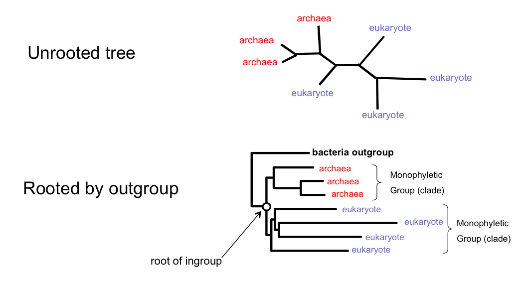
• Monophyletic groups (clades): Groups containing species more closely related to each other than to any species outside the group
• Statistical inference: Modern phylogenetics uses probabilistic models of evolution

A Typical Phylogenetic Analysis

1. Collect homologous sequences - Identify sequences that share common ancestry
2. Construct multiple sequence alignment - Align sequences to identify homologous positions
3. Phylogeny reconstruction - Infer the tree using various methods
4. Test reliability - Assess confidence in the estimated phylogeny
5. Interpretation and application - Use the phylogeny to answer biological questions

Applications of Phylogenetics

Phylogenetic methods have diverse applications across biology:

• Inferring relationships among species and genes
• Estimating divergence times
• Identifying functional elements through comparative genomics
• Detecting molecular adaptation
• Forensics and paternity testing
• Studying the emergence and spread of viral pandemics
• Conservation biology and biodiversity assessment

2. Types and Anatomy of Phylogenetic Trees

Tree Representations

Different ways to represent the same phylogenetic relationships

Phylogenetic trees can be drawn in various formats:

• Rectangular (dendogram): Branch lengths shown horizontally
• Circular: Taxa arranged in a circle
• Radial: Branches radiate from center

Bifurcating vs. Multifurcating Trees

Comparison of fully resolved (bifurcating) and partially resolved (multifurcating) trees

Rooted vs. Unrooted Trees

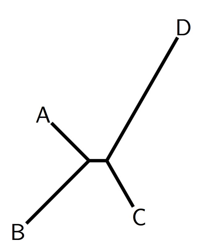
The same evolutionary relationships shown as rooted and unrooted trees

Key differences:

• Rooted trees show the direction of evolution and identify the common ancestor
• Unrooted trees show relationships but not evolutionary direction
• Many methods (parsimony, distance, likelihood without molecular clock) produce unrooted trees

Rooting Trees Using an Outgroup

Using an outgroup (distantly related species) to determine the root position

Tree Anatomy

Key components of a phylogenetic tree

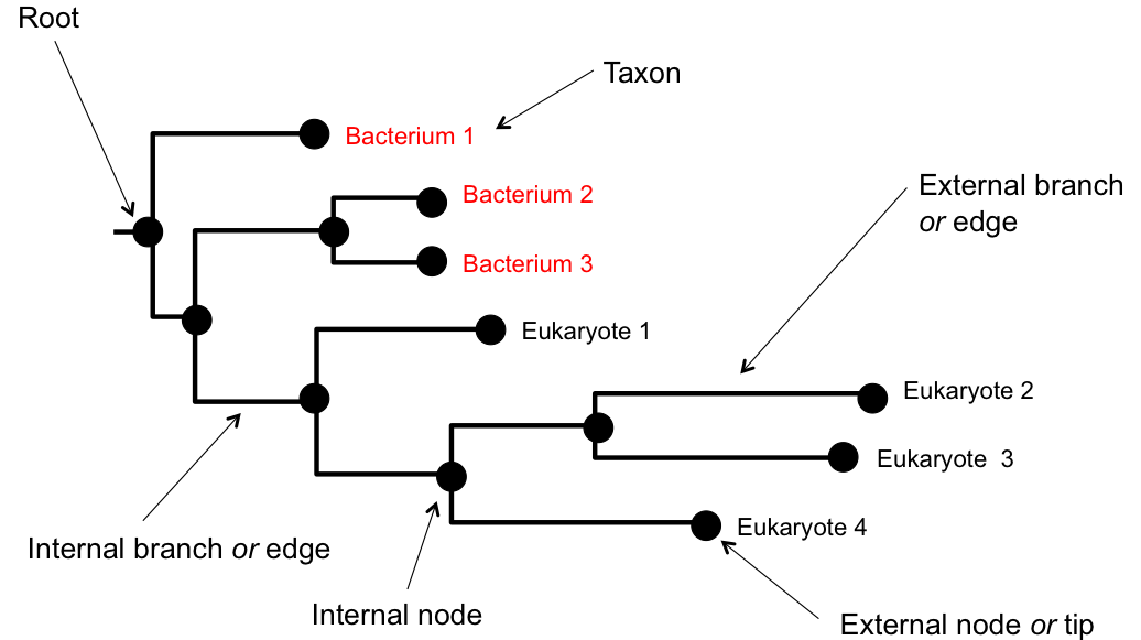
Essential tree terminology:

• Nodes: Points where branches meet (internal nodes = ancestors, tips/leaves = observed taxa)
• Branches/Edges: Lines connecting nodes (represent evolutionary lineages)
• Branch lengths: Can represent time or amount of evolutionary change
• Root: The common ancestor of all taxa in the tree
• Tips/Leaves: The observed taxa (species, genes, etc.)

3. The Universe of Possible Trees

How Many Trees Are There?

The number of possible tree topologies grows explosively with the number of taxa. For $n$ taxa, the number of:

Counting Unrooted Trees

Building trees by stepwise addition shows how tree numbers grow

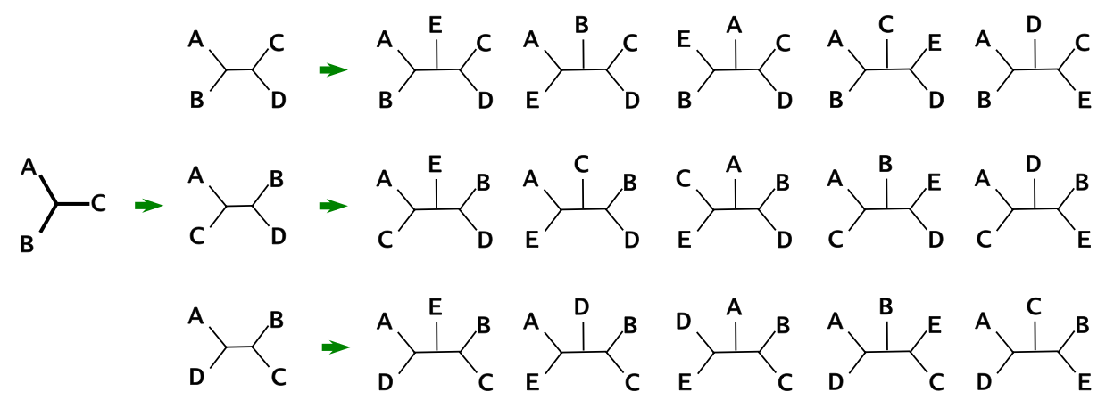
The number of unrooted trees can be calculated using stepwise addition:

• Start with 3 taxa: only 1 possible unrooted tree
• Each new taxon can be added to any branch
• Formula: $T_n = 1 × 3 × 5 × \cdots × (2n-5)$ for $n$ taxa

Measuring Tree Differences

Each internal branch defines a bipartition of taxa. The RF distance counts non-shared bipartitions.

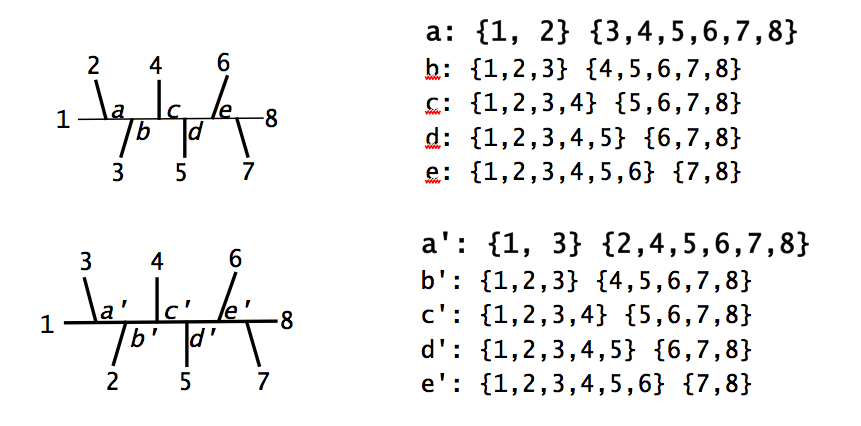
Properties of the Robinson-Foulds distance:

• Ranges from 0 (identical trees) to $2(n-3)$ for $n$ taxa
• Simple to compute but can be sensitive to small changes
• Treats all bipartitions equally (no weighting by branch length)

4. Overview of Phylogenetic Reconstruction

Types of Data

Phylogenetic reconstruction uses two main types of data:

Reconstruction Approaches

Overview of major phylogenetic reconstruction approaches

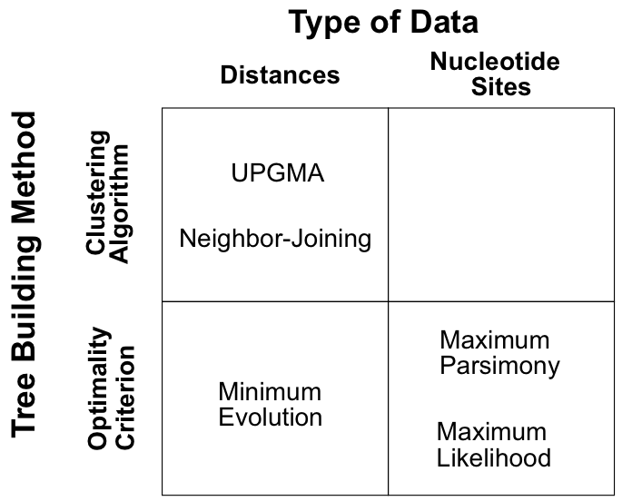
Given the enormous number of possible trees, we have three main strategies:

1. Clustering algorithms: Build tree using a specific algorithm (fast but no optimality criterion)
2. Optimality criteria: Define a score and find the tree(s) that optimize it
3. Statistical inference: Find the most probable trees under an evolutionary model

5. Clustering Methods

Overview of Clustering Approaches

Clustering algorithms like UPGMA and Neighbor-Joining are:

• Usually very fast (polynomial time)
• Simple to implement and understand
• Based on greedy heuristics (make locally optimal choices)

UPGMA (Unweighted Pair Group Method with Arithmetic Mean)

UPGMA is one of the simplest tree-building methods:

UPGMA Example

Final UPGMA tree showing ultrametric property (all leaves equidistant from root)

UPGMA Weaknesses

UPGMA can fail when evolutionary rates vary:

A non-clock-like tree with different topology that fits the distance matrix perfectly

Neighbor-Joining (NJ) Algorithm

Saitou and Nei (1987) developed NJ to address UPGMA's limitations:

The NJ Algorithm

1. Compute "average distance" for each taxon:
   $$r_i = \frac{1}{n-2} \sum_j d_{ij}$$
2. Calculate corrected distances:
   $$d_{ij}^* = d_{ij} - r_i - r_j$$
3. Join the pair with smallest $d_{ij}^*$
4. Calculate branch lengths to new node:
   $$d_{ik} = \frac{1}{2}(d_{ij} + r_i - r_j)$$

NJ correctly groups AB and CD, unlike UPGMA which incorrectly grouped AC

Time Complexity

Both UPGMA and NJ have $O(n^3)$ time complexity:

• $n$ steps (joining operations)
• Each step requires finding minimum distance: $O(n^2)$
• Updating distances: $O(n)$

6. Least Squares Distance Methods

Unlike clustering methods, least squares approaches have an explicit optimality criterion: minimize the difference between observed and tree-implied distances.

The Least Squares Criterion

For any tree topology with branch lengths, we can calculate the sum of squared differences:

Where:

• $d_{ij}$ = observed distance between taxa $i$ and $j$
• $\hat{d}_{ij}$ = tree-implied distance (sum of branch lengths on path)

Tree-implied distances are sums of branch lengths along paths

Optimization Process

For the primate example:

• 6 data points (pairwise distances)
• 5 free parameters (branch lengths)
• Use numerical optimization to minimize $S$

Different tree topologies with optimized branch lengths and their fit to the data

Advantages and Limitations

Advantages:

• Explicit optimality criterion
• Can compare different topologies
• Provides branch length estimates

Limitations:

• Still need to search tree space (NP-hard problem)
• Assumes distances are measured without error
• No statistical framework for uncertainty

Summary

This lecture introduced the fundamentals of phylogenetic analysis:

1. Evolutionary information: Molecular sequences contain historical information that can be decoded through phylogenetic analysis
2. Tree basics: Understanding tree anatomy, rooted vs. unrooted trees, and different representations
3. Tree space: The number of possible trees grows explosively, making exhaustive searches impossible
4. Distance methods:
   • Clustering (UPGMA, NJ): Fast but no optimality measure
   • Least squares: Explicit criterion but computationally intensive
5. Key challenges: Accounting for rate variation, searching vast tree space, and quantifying uncertainty