Sequence Homology

1. Introduction to Sequence Homology

Understanding homology is fundamental to phylogenetic analysis. When we observe similarity between sequences, we form hypotheses about their evolutionary relationships.

Key Concepts

• Homologous sequence regions are expected to display a degree of similarity
• The statement that two sequence regions are homologous is an evolutionary hypothesis based on similarity
• It is rarely possible to observe homology directly
• Homologous sequences are referred to as homologs

Types of Homologs

Different evolutionary events can lead to different types of homologous relationships:

• Orthology: Ancestral sequences separated by speciation
• Paralogy: Ancestral sequences separated by gene duplication
• Xenology: Homologs resulting from horizontal gene transfer

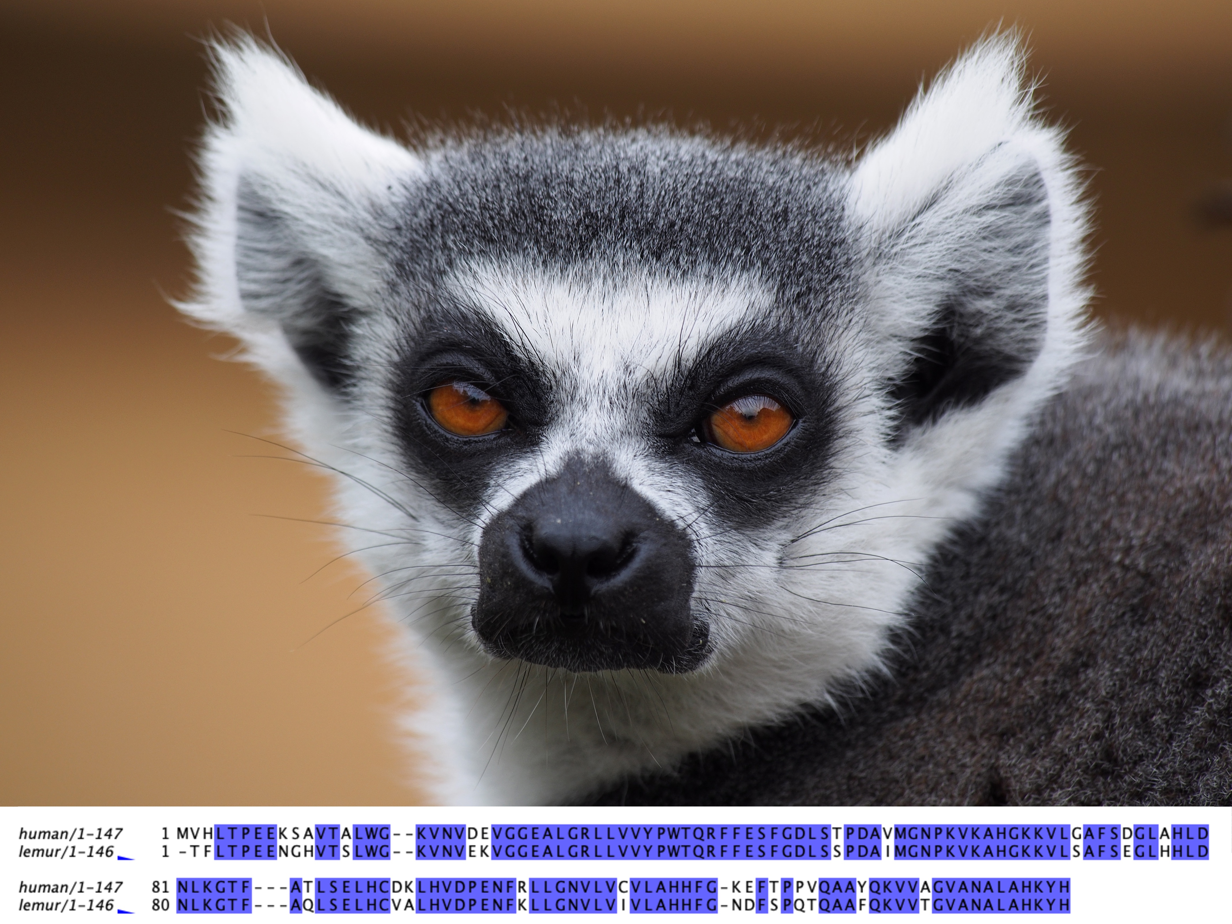
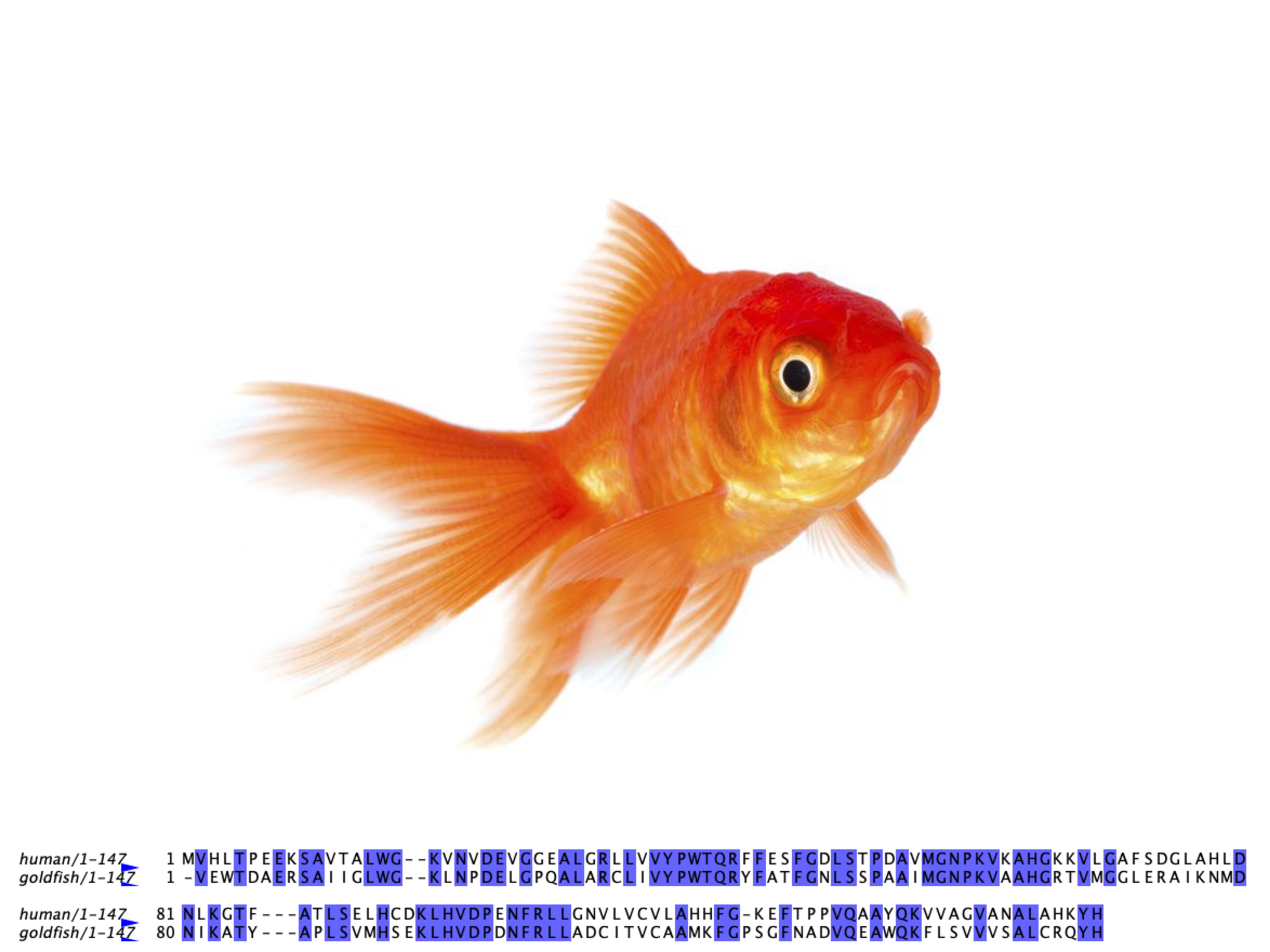
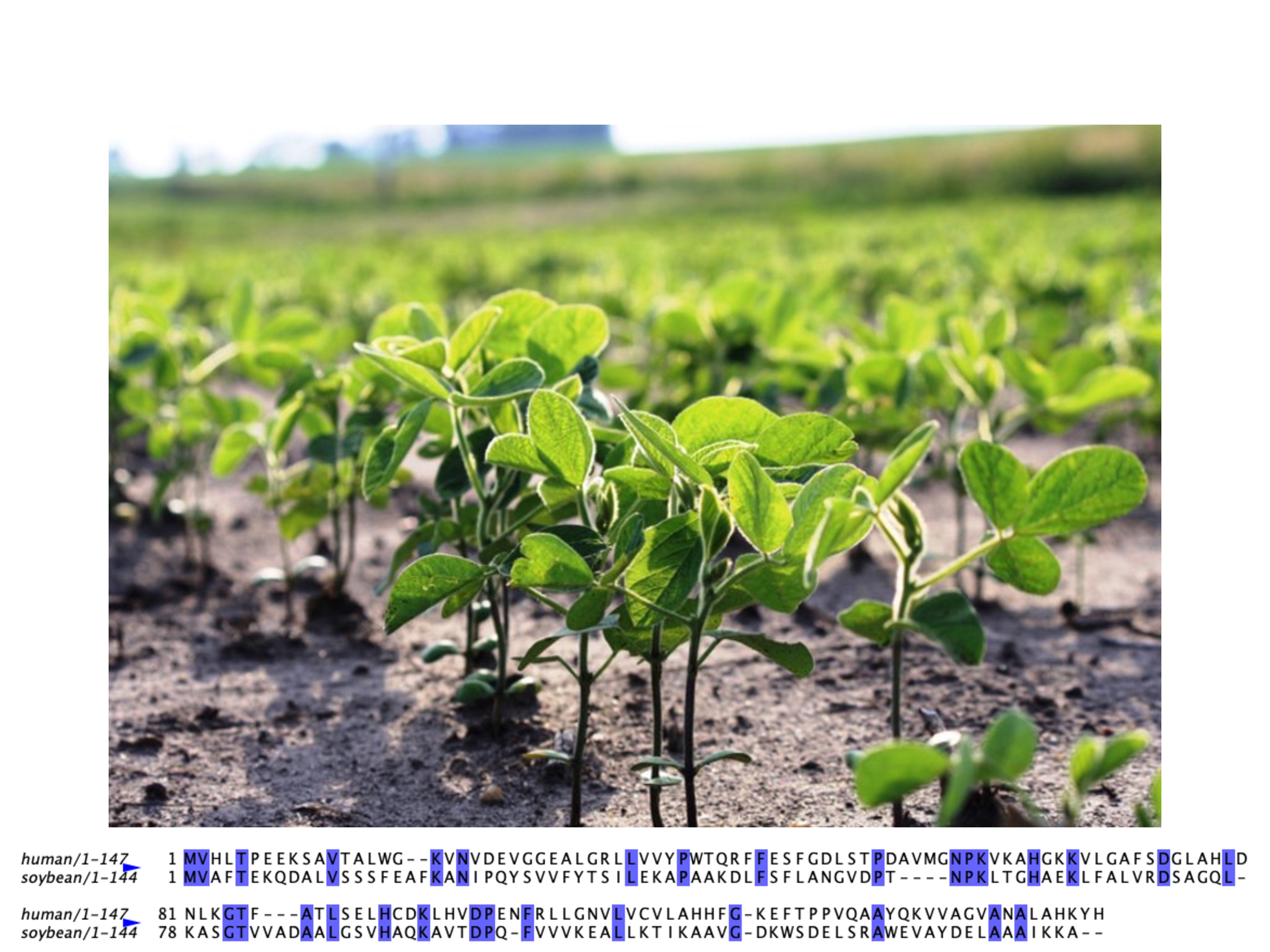
Examples from Nature

The globin family provides excellent examples of homologous proteins across diverse organisms:

Ring-tailed lemur beta globin structure

Goldfish beta globin structure

Soybean leghemoglobin structure

2. Pairwise Alignment

The Goal of Pairwise Alignment

Aligning one sequence with another allows us to assess the homology between the two sequences.

Alignment serves several crucial purposes in sequence analysis:

• It breaks down the question of sequence similarity into smaller questions about character similarity
• It forms the basis for multiple sequence alignment
• It provides the foundation for phylogenetic reconstruction from molecular data

Dot Plots

A simple visual method for assessing pairwise homology. Consider these two sequences:

1. "decided to build three ships, three Arks in space"
2. "decided to build three Arks in space"

Dot plot showing diagonal lines indicating runs of matching sites

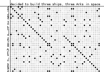
• Each row corresponds to a position on sequence 1
• Each column corresponds to a position on sequence 2
• Pixel (i,j) is colored if characters at site i on seq 1 and j on seq 2 match
• Diagonal lines indicate runs of matching sites

Scoring Alignments

Alignments are evaluated using scoring systems that assign numeric values to each column:

Column types and their typical scores:

• Identical: Positive score
• Conservative: Positive score
• Non-conservative: Negative score
• Gap: Negative score

Scoring Methods

Two main approaches are used for scoring alignments:

1. Model-based Scoring

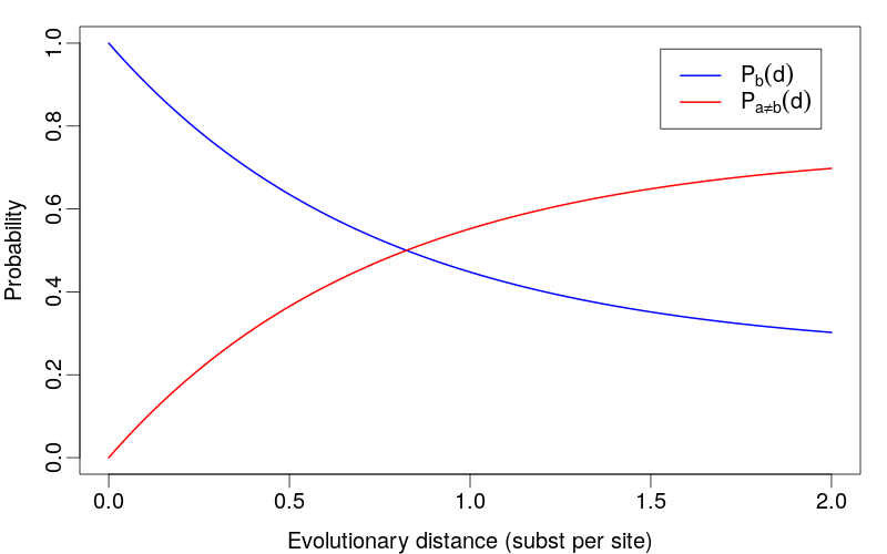
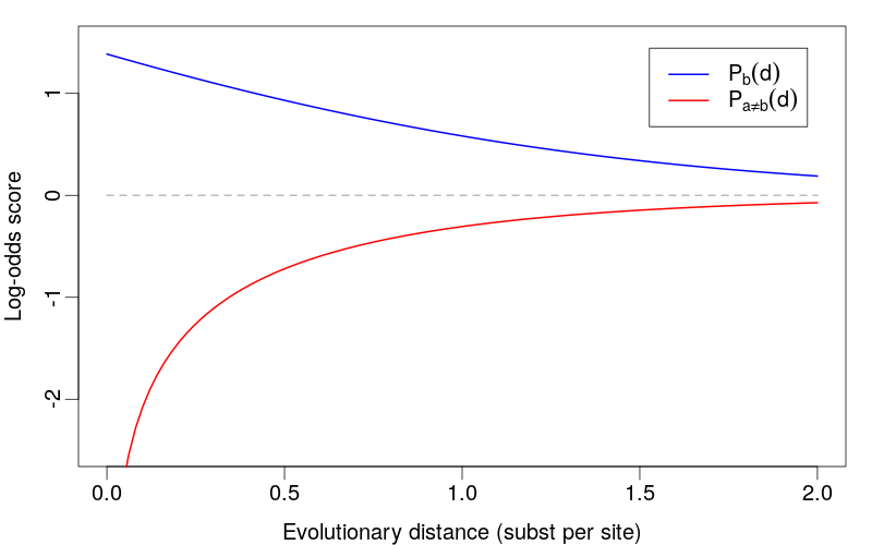
Based on evolutionary models, particularly log-odds scoring:

Where:

• \(p_{ab}\) is the probability of observing residues a and b in homologous sequences
• \(f_a\) and \(f_b\) are the background frequencies of residues a and b
• \(\lambda\) is a scaling factor

2. Empirical Scoring

Based on observed substitution patterns in real sequences:

• PAM matrices
• BLOSUM matrices
• JTT matrix
• WAG matrix

Evolutionary Interpretation

For homologous sequences with divergence time \(t\) and mutation rate \(\mu\):

Variation of match/mismatch probabilities with evolutionary distance \(d = \mu t\)

Variation of match/mismatch scores with evolutionary distance

Gap Penalties

Illustration of gap penalties in sequence alignment

Two main approaches for penalizing gaps in alignments:

1. Linear gap penalty:
   $$\gamma(g) = -gd$$
   where \(d\) is the gap penalty and \(g\) is the gap length
2. Affine gap penalty:
   $$\gamma(g) = -d - (g-1)e$$
   where \(d\) is the gap opening penalty and \(e\) is the gap extension penalty

3. Pairwise Alignment Algorithms

Dynamic Programming

Dynamic programming is a powerful method for solving combinatorial optimization problems. It guarantees finding the optimal solution and is based on the principle of optimality:

A sub-optimal solution of a sub-problem cannot be part of the optimal solution of the full problem.

Illustration of the principle of optimality in dynamic programming

Key features of dynamic programming:

• Computation is carried out from the bottom-up
• All solutions to sub-problems are stored in a table
• Each sub-problem is solved exactly once
• Only optimal solutions to sub-problems are used for the next level

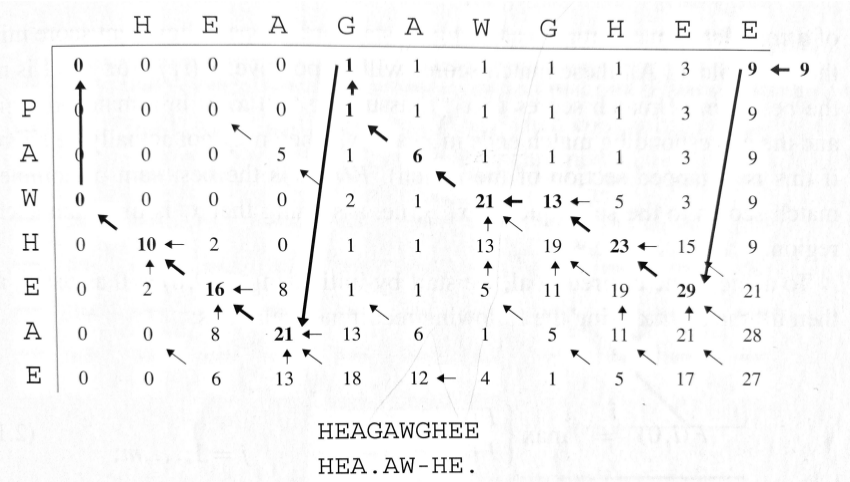
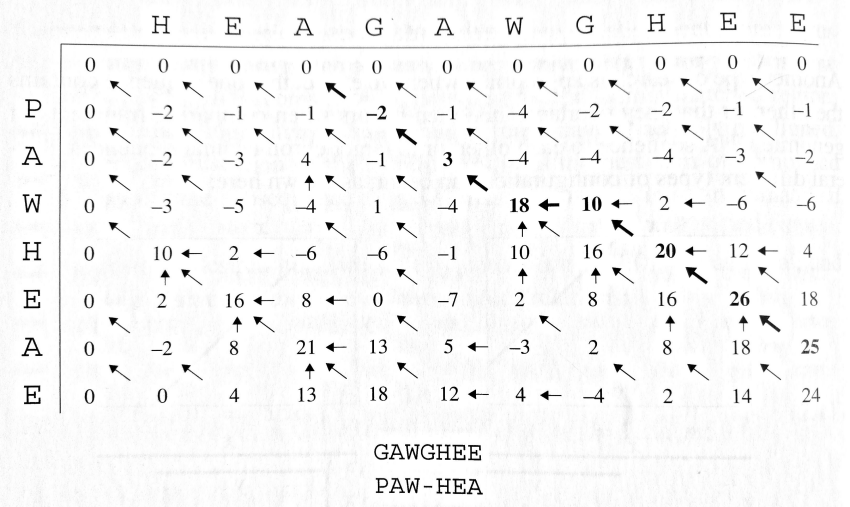
Needleman-Wunsch Algorithm

The Needleman-Wunsch algorithm (1970) performs global alignment using dynamic programming.

Algorithm Overview

Given sequences X = (x₁, x₂, ..., xₘ) and Y = (y₁, y₂, ..., yₙ), where m and n are the lengths of sequences X and Y respectively, define F(i,j) as the score of the best alignment between the first i characters of X and the first j characters of Y.

Recurrence Relation

Initialization

• F(0,0) = 0
• F(i,0) = F(i-1,0) + s(xᵢ,-) for i > 0
• F(0,j) = F(0,j-1) + s(-,yⱼ) for j > 0

Smith-Waterman Algorithm

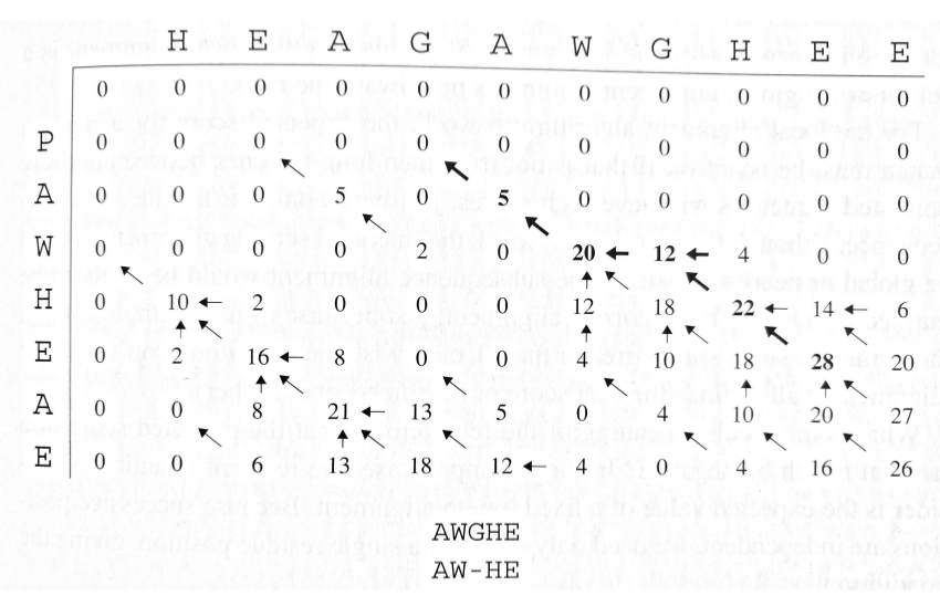
The Smith-Waterman algorithm computes local alignment, finding the best alignment of subsequences while ignoring scores of regions on either side.

Local alignment finds high-scoring subsequences

Key Difference

The main difference from Needleman-Wunsch is the addition of a fourth option in the recurrence:

This allows the algorithm to:

• Start a new alignment at any position
• End an alignment when the score becomes negative
• Find multiple high-scoring local alignments

Example of Smith-Waterman algorithm finding local alignments

Specialized Variants

Repeated Matches

For finding multiple occurrences of a motif in a longer sequence:

• Useful for identifying repeated domains or motifs
• Asymmetric algorithm (short query vs. long target)
• Tracks multiple high-scoring regions above threshold T

Finding repeated motifs using modified dynamic programming

Overlap Matches

For sequence assembly and finding overlapping sequences:

• No penalty for overhanging ends: F(i,0) = F(0,j) = 0
• Useful in genome assembly projects
• Identifies sequences that overlap at their ends

Overlap alignment for sequence assembly

Summary and Next Steps

In this lecture, we've covered the fundamental concepts of sequence homology and pairwise alignment:

• The definition and types of homology
• Methods for visualizing and scoring sequence alignments
• Dynamic programming algorithms for global and local alignment
• Specialized alignment variants for specific biological problems

These concepts form the foundation for:

• Multiple sequence alignment (next lecture)
• Phylogenetic tree construction
• Evolutionary rate estimation
• Functional annotation of sequences