The Coalescent - Bayesian phylogenetics lectures

1. Introduction to the Coalescent

The coalescent is one of the most important theoretical frameworks in population genetics and molecular evolution. It provides a mathematical description of how genetic lineages merge backward in time.

The Coalescent

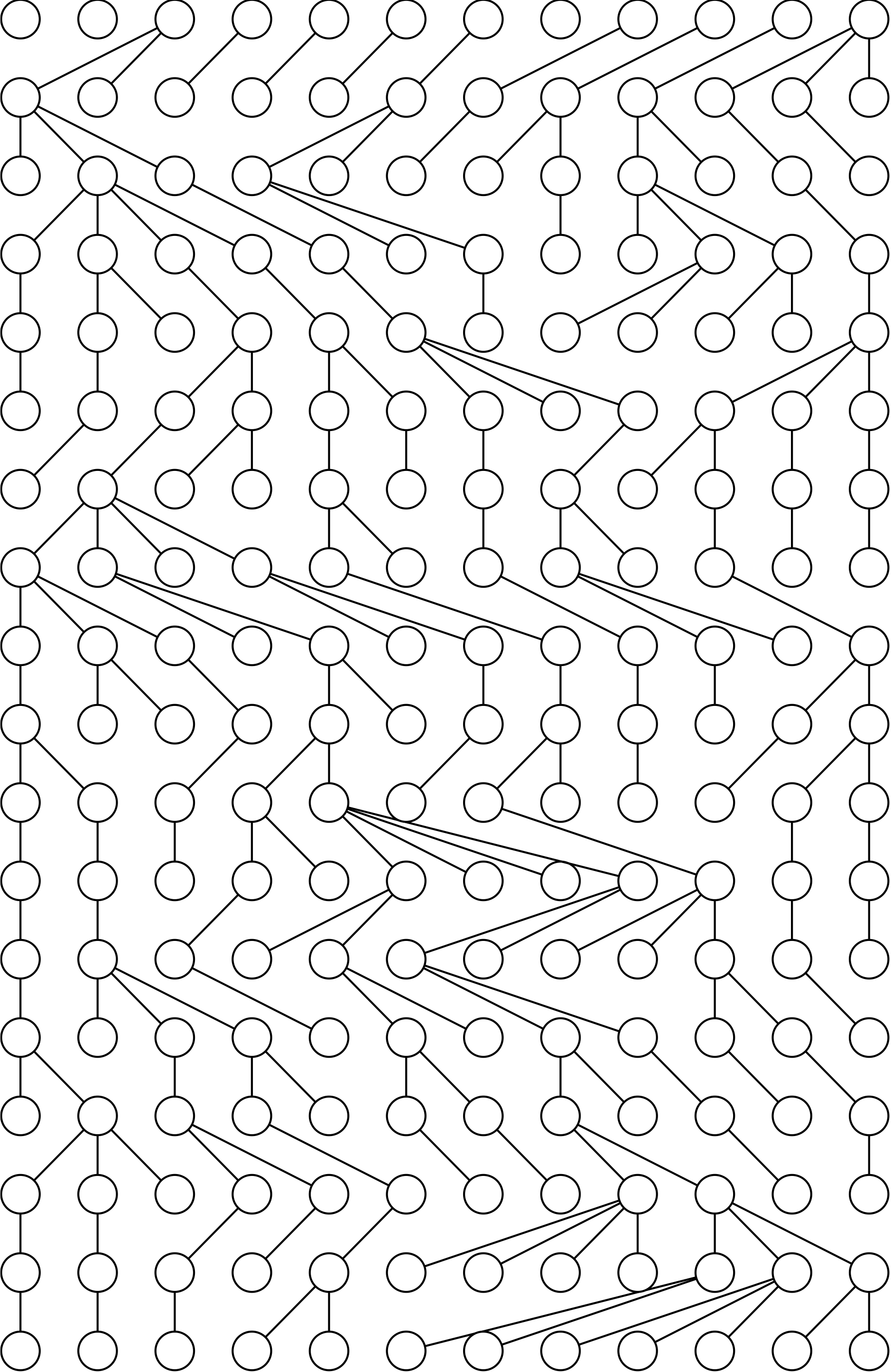
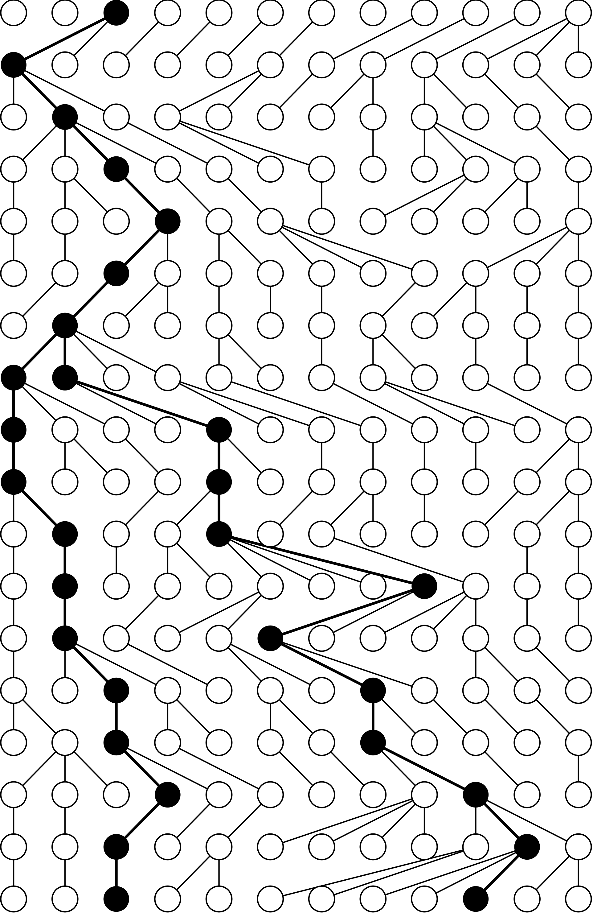
Data: a small genetic sample from a large background population

The coalescent:

Is a model of the ancestral relationships of a sample of individuals taken from a larger population
Describes a probability distribution on ancestral genealogies (trees) given a population history, N(t)
Can convert information from ancestral genealogies into information about population history and vice versa
Is a model of ancestral genealogies, not sequences, and its simplest form assumes neutral evolution
Can be thought of as a prior on the tree, in a Bayesian setting

Key insight: The coalescent allows us to link observable patterns in genetic data to the demographic history of populations.

Why the Coalescent Matters

The coalescent framework is crucial because it:

Provides a null model for genetic variation under neutrality
Enables inference of population parameters from genetic data
Forms the basis for many modern population genetic analyses
Connects microevolutionary processes to macroevolutionary patterns

2. Theoretical Population Genetics Foundation

The Wright-Fisher Model

Most of theoretical population genetics is based on the idealized Wright-Fisher model of population, which makes several simplifying assumptions:

Wright-Fisher Model Assumptions

Constant population size N
Discrete generations (no overlapping generations)
Complete mixing (random mating)
Neutral evolution (no selection)
No mutation (in the basic model)
No migration (closed population)

The Wright-Fisher model: each generation is formed by random sampling with replacement from the previous generation

Note: For the purposes of this presentation, the population will be assumed to be haploid, as is the case for many pathogens. The diploid case follows similar principles with adjusted parameters.

From Forward to Backward in Time

Traditional population genetics works forward in time, tracking allele frequencies through generations. The coalescent takes a different approach:

Forward in time: Track all individuals and their descendants
Backward in time: Track only the ancestors of the sample

This backward-time approach is computationally efficient because:

We only track lineages that contribute to the present-day sample
The number of lineages decreases as we go back in time
We can ignore the vast majority of the population that left no descendants in our sample

3. Kingman's n-Coalescent

John Kingman's groundbreaking work in 1982 established the mathematical foundation for coalescent theory.

Kingman's n-Coalescent

Consider tracing the ancestry of a sample of $k$ individuals from the present, back into the past. This process eventually coalesces to a single common ancestor (concestor) of the sample.

Kingman's n-coalescent describes the statistical properties of such an ancestry when $k$ is small compared to the total population size $N$.

Tracing lineages backward in time until they coalesce to a common ancestor

The Coalescence of Two Lineages

Let's start with the simplest case: two randomly sampled individuals from a population of size $N$.

Two-Lineage Coalescence

By perfect mixing, the probability they share a common ancestor in the previous generation is $1/N$
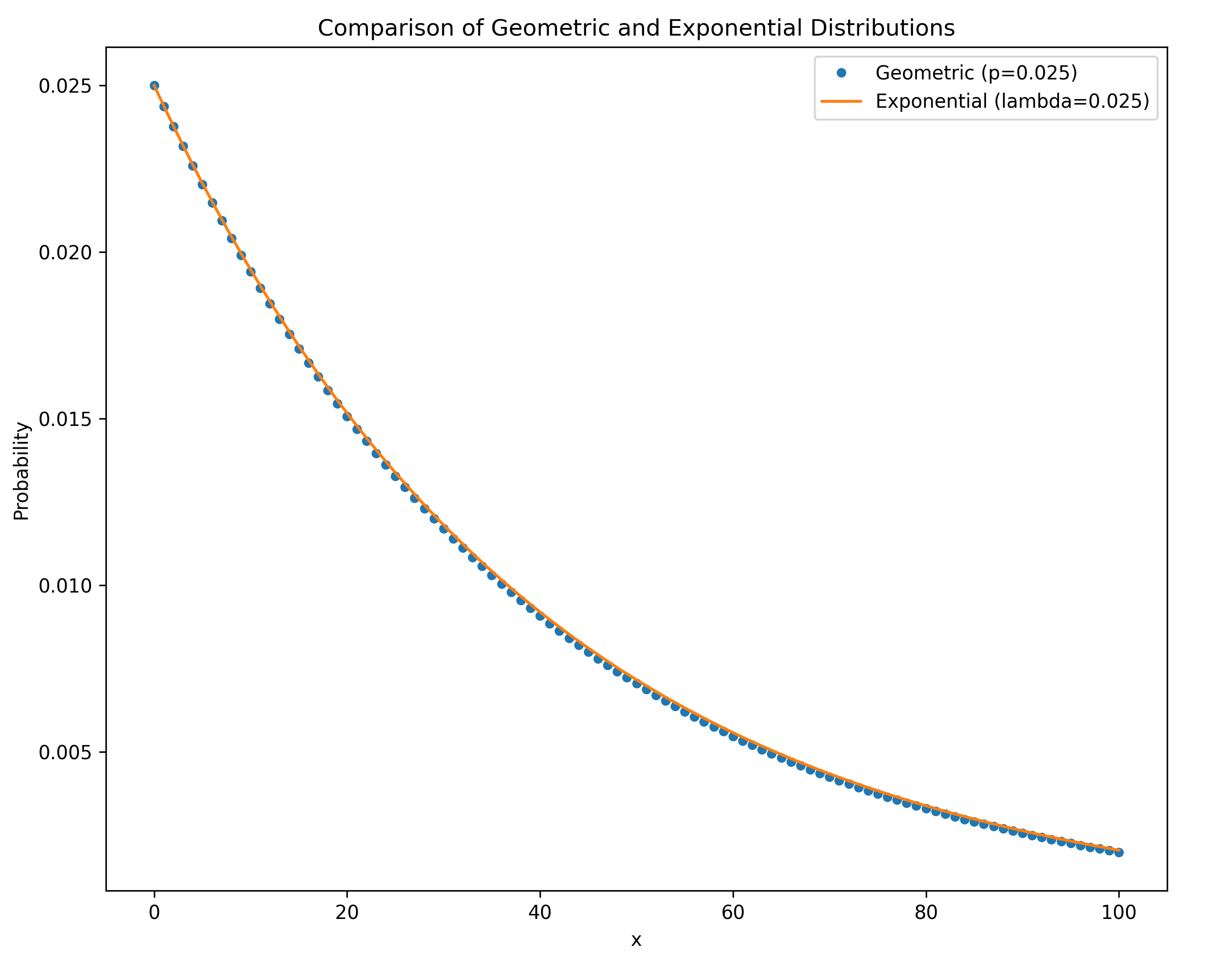
The probability the common ancestor is $t$ generations back is: $P(t) = \frac{1}{N}\left(1-\frac{1}{N}\right)^{t-1}$
This is a geometric distribution with success rate $\lambda = 1/N$
Mean time to coalescence: $E[t] = N$ generations
Variance: $\text{Var}[t] = N^2(1-1/N) \approx N^2$ for large $N$

Two lineages coalescing in the Wright-Fisher model

The Coalescence of k Lineages

With $k$ lineages, the analysis becomes more complex but follows similar principles:

k-Lineage Coalescence

With $k$ lineages, there are $\binom{k}{2} = \frac{k(k-1)}{2}$ possible pairs that may coalesce.

Coalescence rate: $\lambda_k = \binom{k}{2}/N$
Mean time to first coalescence: $E[t_k] = \frac{N}{\binom{k}{2}} = \frac{2N}{k(k-1)}$
After coalescence, we have $k-1$ lineages remaining

Important assumption: This implicitly assumes that $N$ is much larger than $O(k^2)$, so that the probability of two coalescent events in the same generation is negligible.

The Complete Coalescent Process

The complete coalescent process for a sample of $n$ individuals involves successive coalescence events:

Lineages	Coalescence Rate	Expected Time
$n → n-1$	$\binom{n}{2}/N$	$\frac{2N}{n(n-1)}$
$n-1 → n-2$	$\binom{n-1}{2}/N$	$\frac{2N}{(n-1)(n-2)}$
...	...	...
$3 → 2$	$3/N$	$N/3$
$2 → 1$	$1/N$	$N$

Total expected time to the most recent common ancestor (TMRCA):

E[T_{MRCA}] = 2N\sum_{k=2}^n \frac{1}{k(k-1)} = 2N\left(1 - \frac{1}{n}\right)

Key result: As $n → ∞$, $E[T_{MRCA}] → 2N$. The expected TMRCA approaches $2N$ generations regardless of sample size!

4. The Coalescent as a Continuous-Time Process

From Discrete to Continuous Time

As the population size $N$ becomes large, the discrete-time Wright-Fisher model converges to a continuous-time process:

The geometric distribution converges to the exponential distribution as population size increases

The Coalescent as a Diffusion Approximation

Kingman (1982) showed that as $N$ grows, the coalescent process converges to a continuous-time Markov chain.

Continuous-Time Coalescent

For $k$ lineages, the waiting time until the next coalescence follows an exponential distribution:

f(t_k) = \frac{\binom{k}{2}}{N}\exp\left(-\frac{\binom{k}{2}t_k}{N}\right)

For a specific pair of lineages to coalesce:

f(t_k) = \frac{1}{N}\exp\left(-\frac{\binom{k}{2}t_k}{N}\right)

From Wright-Fisher genealogy to coalescent tree representation

5. The Coalescent Density

Probability Density for a Genealogy

For a genealogy $g$ with $n$ samples and coalescent times $\mathbf{t} = \{t_2, t_3, \ldots, t_n\}$, we can write the probability density:

Coalescent Density Function

P(g|N) = \frac{1}{N^{n-1}}\prod_{k=2}^n\exp\left(-\frac{\binom{k}{2}t_k}{N}\right)

Where:

$t_k$ is the time interval during which there are $k$ lineages
The factor $1/N$ appears for each coalescence event (probability of specific pair coalescing)
The exponential term accounts for the waiting time with $k$ lineages

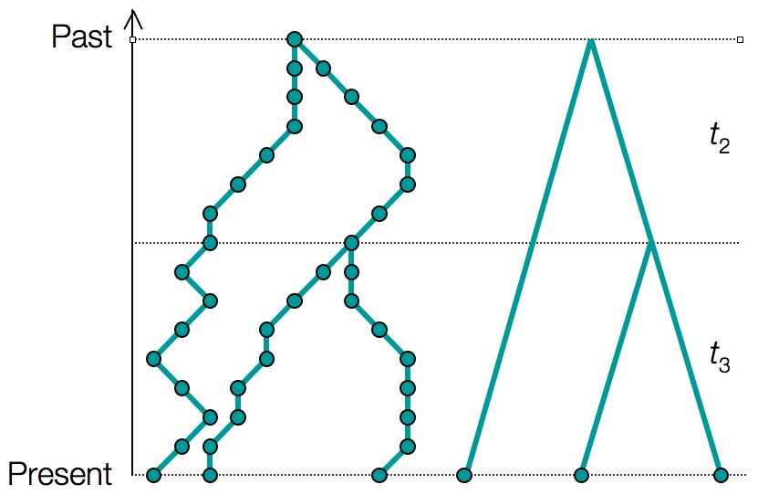
Example: Three-Sample Genealogy

For $n = 3$ samples with coalescence times $t_3$ (3→2 lineages) and $t_2$ (2→1 lineages):

P(g|N) = \frac{1}{N^2} \exp\left(-\frac{3t_3}{N}\right) \exp\left(-\frac{t_2}{N}\right)

This shows how both topology and branch lengths contribute to the genealogy probability.

Properties of the Coalescent Density

Factorization: The density factorizes over coalescence intervals
Markov property: Given $k$ lineages, future coalescence is independent of past
Exchangeability: All labeled topologies are equally likely under the standard coalescent

6. The Coalescent with Variable Population Size

Real populations rarely maintain constant size. The coalescent can be generalized to handle time-varying population sizes.

Variable Population Size Coalescent

Griffiths and Tavaré (1994) showed that for population size $N(t)$ varying with time:

Coalescent Density with Variable N(t)

The probability density for the first coalescence event at time $t$ given $n$ lineages:

f(t) = \frac{\binom{n}{2}}{N(t)} \exp\left(-\int_0^t \frac{\binom{n}{2}}{N(x)} dx\right)

Requirements:

The coalescent intensity function $1/N(t)$ must be integrable
$N(t) > 0$ for all $t$

Common Population Size Functions

Examples of N(t)

1. Exponential growth/decline:

N(t) = N_0 e^{-rt}

2. Logistic growth:

N(t) = \frac{K}{1 + \left(\frac{K}{N_0} - 1\right)e^{-rt}}

3. Bottleneck:

N(t) = \begin{cases} N_0 & \text{if } t < t_b \text{ or } t > t_b + \Delta t \\ N_b & \text{if } t_b \leq t \leq t_b + \Delta t \end{cases}

Effects of Population Size Changes

Different demographic scenarios leave characteristic signatures in genealogies:

Population expansion: Star-like trees with long terminal branches
Population bottleneck: Rapid coalescence during the bottleneck
Cyclic population size: Clustering of coalescence events

Key insight: The shape of a genealogy contains information about historical population size changes. This is the basis for demographic inference from genetic data.

7. Applications and Extensions

The Coalescent as a Tree Prior

In Bayesian phylogenetics, the coalescent serves as a natural prior distribution on gene trees:

P(\text{tree}|\theta)

Where $\theta$ includes parameters like:

Effective population size $N_e$
Growth rate $r$
Migration rates (for structured populations)

Extensions of the Basic Coalescent

Structured Coalescent: Accounts for population subdivision and migration
Selection at Linked Sites: Modifies coalescence rates due to hitchhiking effects
Recombination: Leads to the ancestral recombination graph (ARG)
Multiple Merger Coalescents: Allows more than two lineages to coalesce simultaneously

Practical Applications

The coalescent framework enables:

Demographic inference: Estimating historical population sizes and growth rates
Species delimitation: Distinguishing population structure from species boundaries
Dating events: Estimating times of population splits or admixture
Selection detection: Identifying deviations from neutral expectations
Epidemiological inference: Tracking pathogen spread and transmission

Software Implementing Coalescent Models

BEAST/BEAST2: Bayesian phylogenetics with coalescent priors
MIGRATE: Estimation of migration rates and population sizes
ms/msprime: Coalescent simulation programs
LAMARC: Likelihood analysis with coalescent models
IMa2: Isolation with migration models

8. Visualizing the Coalescent Process

Understanding the coalescent often benefits from visualization and simulation. The interactive demonstration in the lecture allows exploration of:

Key Parameters to Explore

Sample size (n): How does increasing n affect the genealogy shape?
Population size (N): How does N affect coalescence rate?
Population dynamics: Effects of different N(t) functions:
- Sinusoidal (cyclic populations)
- Square wave (abrupt changes)
- Sawtooth (gradual change followed by crash)

Observable Patterns

Through simulation, we can observe:

The randomness in coalescence times and tree shapes
How bottlenecks accelerate coalescence
The relationship between N(t) and the coalescent density
Why most coalescence occurs near the present (for constant N)

Exercise: Try simulating genealogies with different population size functions. Notice how bottlenecks create "hourglass" shaped genealogies, while expansion creates "star" phylogenies.

Summary

The coalescent is a fundamental framework in population genetics that:

Provides a null model: Describes genealogies under neutral evolution in idealized populations
Works backward in time: More efficient than forward simulations for genealogical questions
Links demography to genealogy: Population size changes leave signatures in gene trees
Has elegant mathematics:
- Exponential waiting times between coalescence events
- Rate depends on number of lineages and population size
- Generalizes to variable population sizes
Forms the basis for inference: Used as tree priors in Bayesian phylogenetics and for demographic inference
Has many extensions: Can incorporate population structure, selection, recombination, and other biological realities

Key formula to remember: For $k$ lineages in a population of size $N$, the rate of coalescence is $\binom{k}{2}/N$, and the expected waiting time is $N/\binom{k}{2}$.

Recommended Reading:

Wakeley (2009) "Coalescent Theory: An Introduction" - Chapters 1-3
Hein, Schierup & Wiuf (2005) "Gene Genealogies, Variation and Evolution" - Chapters 3-4
Kingman (1982) "The coalescent" - Stochastic Processes and their Applications
Griffiths & Tavaré (1994) "Sampling theory for neutral alleles" - Phil Trans R Soc B

Check Your Understanding

Why is the coalescent more efficient than forward-time simulations?
What is the expected TMRCA for a large sample from a population of size N?
How does a population bottleneck affect the rate of coalescence?
Why do all labeled topologies have equal probability under the standard coalescent?
What information about population history can be inferred from genealogy shape?