Molecular clocks and dated phylogenies
The question this lecture answers
A phylogeny with a calendar axis tells you when lineages last shared an ancestor. That is what turns a tree into a statement about history: when a virus entered a country, when two species diverged, how old a fossil lineage is.
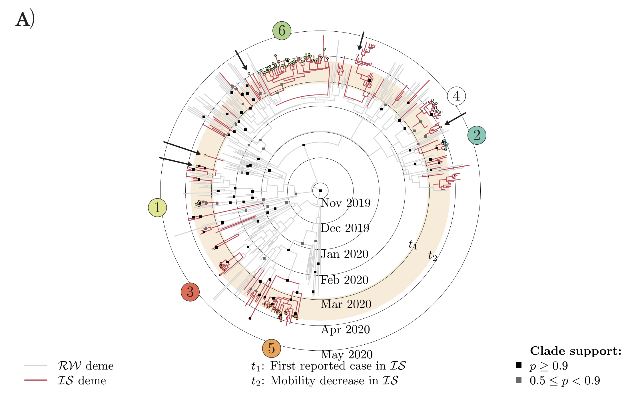
The sample dates at the tips are known. Every internal date is estimated, and so has a posterior distribution and a credible interval, exactly like any other parameter from L8. The squares are posterior clade probabilities.
1. The Molecular Clock Hypothesis
Genetic Distance = Rate × Time
The fundamental equation of molecular evolution:
The Molecular Clock Equation
Where:
- $d$ = genetic distance (expected substitutions per site)
- $\mu$ = substitution rate (substitutions per site per unit time)
- $t$ = time
The Strict Molecular Clock
Under a strict molecular clock, all lineages evolve at the same rate:

- Single evolutionary rate $\mu$ for all branches
- Ultrametric trees (all tips equidistant from root)
- Proposed by Zuckerkandl and Pauling (1962)
- Enables dating without fossils if rate is known
2. The Identifiability Problem
Non-identifiability of Rate and Time

Solutions to the Identifiability Problem
To separate rate and time, we need additional information:
1. Node Calibrations
Use fossil or biogeographic evidence to constrain node ages:

Node Calibration in Practice
- Fossil provides minimum age (fossil must be younger than clade)
- Biogeography can provide maximum age (e.g., island age)
- Often specified as probability distributions (e.g., lognormal)
- Multiple calibrations improve precision
2. Tip Calibrations
Use samples from different time points:

Applications of Tip Calibration
- Ancient DNA: Subfossil remains, museum specimens
- Rapidly evolving pathogens: Virus samples from different years
- Laboratory evolution: Samples from known time points
3. Relaxed Molecular Clocks
The strict molecular clock is often too restrictive. Relaxed clocks allow rate variation across branches.
Relaxed Clock Parameterization

Instead of a single rate $\mu$, we have a vector of rates $\vec{\mu} = (\mu_1, \mu_2, ..., \mu_{2n-2})$
The substitution tree is computed as: $T = \vec{\mu} \star g$
Where $\star$ denotes element-wise multiplication of rates and branch durations
Identifiability Under Relaxed Clocks

4. Bayesian Framework for Molecular Clocks
Posterior with Strict Clock
Strict Clock Posterior
Substitution tree: $T = \color{darkgreen}{\mu} \times \color{red}{g}$
Where:
- $\color{red}{g}$ = time tree
- $\color{darkgreen}{\mu}$ = clock rate
- $\color{blue}{\Theta}$ = tree prior parameters (as in L7 and L8)
Posterior with Relaxed Clock
Relaxed Clock Posterior
Substitution tree: $T = \color{darkgreen}{\vec{\mu}} \star \color{red}{g}$
Where $P(\color{darkgreen}{\vec{\mu}})$ is the prior for rate variation
- The phylogenetic likelihood only depends on the substitution tree $T$: $\Pr(D|T)$
- The tree prior only depends on the time tree $\color{red}{g}$: $P(\color{red}{g}|\color{blue}{\Theta})$
- By fixing $\color{darkgreen}{\vec{\mu}} = 1$, we get a time tree in units of substitutions
5. Models of Rate Variation
Autocorrelated Models
Rates evolve along the tree, with child rates similar to parent rates:
Common implementation: Lognormal autocorrelated model
Where:
- $t_i$ = time duration of branch $i$
- $\sigma$ = rate of evolution of rates (volatility parameter)
Uncorrelated Models
Rates are drawn independently for each branch:
Common implementations:
- Lognormal: $\log(\mu_i) \sim \text{Normal}(M, S)$
- Exponential: $\mu_i \sim \text{Exponential}(\lambda)$
- Gamma: $\mu_i \sim \text{Gamma}(\alpha, \beta)$
Autocorrelated
- Biologically motivated
- Smooth rate changes
- Good for closely related species
- Can extrapolate rates
Uncorrelated
- More flexible
- Allows sudden rate changes
- Good for diverse datasets
- Simpler to implement
6. Advantages of Molecular Clock Models
Relaxed molecular clocks offer several benefits over unconstrained models:
- Improved phylogenetic accuracy:
- Rate smoothing helps identify correct topology
- Reduces long-branch attraction artifacts
- Better performance on empirical datasets
- Automatic rooting:
- No need for outgroup
- Root position estimated from rate variation
- Particularly useful when outgroup is distant
- Temporal information:
- Relative divergence times always available
- Absolute times with calibration
- Useful for studying evolutionary rates
- Integration with other models:
- Natural combination with coalescent priors
- Enables epidemiological inference
- Links to fossil data
Summary
This lecture answered one question: how do we put a date, with an interval, on a common ancestor?
- The obstacle:
- Sequences record genetic distance, and distance = rate × time
- Rate and time are non-identifiable: a fast rate over a short time and a slow rate over a long time give identical likelihoods
- The solution, calibration:
- Node calibration from a dated fossil
- Tip calibration from samples of different known ages: ancient DNA, or a fast-evolving virus sequenced over months
- Either one puts the whole tree on a scale of years
- Rate variation:
- Strict clocks assume one rate; relaxed clocks give every branch its own
- Relaxed clocks are usually more realistic, but add non-identifiability that only the priors resolve, so priors must be reported
- Uncorrelated draws each rate independently; autocorrelated lets rate evolve along the tree
- What you get out:
- A posterior distribution of dates for every ancestor, hence credible intervals
- A rooted tree without needing an outgroup
- Dates that are conditional on the clock model, substitution model and tree prior
- Stadler et al. (2024) Decoding Genomes - Ch 6.4 (strict clock, time trees, calibrations)
- Drummond & Bouckaert (2015) "Bayesian Evolutionary Analysis with BEAST" - Chapters 6-7 (relaxed clocks in detail)
- Yang (2014) "Molecular Evolution: A Statistical Approach" - Chapter 7
- Drummond et al. (2006) "Relaxed phylogenetics and dating with confidence" - PLOS Biology
- Douglas et al. (2021) "Phylodynamics reveals the role of human travel and contact tracing in controlling the first wave of COVID-19 in four island nations" - Virus Evolution 7(2):veab052. Source of the opening figure.
Check Your Understanding
- What makes rate and time non-identifiable in molecular evolution?
- How do node and tip calibrations solve the identifiability problem?
- The SARS-CoV-2 tree in the opening figure has a calendar axis even though there are no fossils. What calibrates it?
- What's the key difference between autocorrelated and uncorrelated relaxed clocks?
- Why do relaxed clocks often produce better phylogenetic estimates than no-clock models, and what do they make you more dependent on?
- A paper reports a divergence date of 12.4 Mya. What else must it report before you can judge that number?