🏠

Model Selection

Generate layout for printing

Lecturer: Alexei Drummond

All models are wrong.

Some are useful.

(G. E. P. Box, 1979)

How do we tell which?

What today's math is for

Every time you fit a model to biological data, you face a choice:

Phylogeny. JC, K80, HKY, GTR, $+\Gamma$, $+I$, … pick the wrong substitution model and your tree is biased.
Trait evolution. Constant-rate Brownian motion, or an early burst? Or convergence on multiple adaptive peaks? (Next lecture.)
Divergence times. Strict molecular clock, or a relaxed one? The same calibrations can give different node ages depending on how rate variation is modelled across branches.

A bigger model can always fit the observed data better. The question is:

When does an extra parameter improve a model enough to justify its inclusion?

That is what this lecture answers.

Three tools you'll meet today

Likelihood Ratio Test. Nested models only; classical $\chi^2$.
AIC / AIC_c / AIC weights. Any models; graded support.
Bayes Factors. Bayesian; integrates over parameter uncertainty.

Next lecture applies all three to evolutionary trait data, and ends with a paper whose punchline is "$\Delta\mathrm{AIC}_c = 162.6$".

Recall: likelihood and the MLE

From the substitution models lecture (Week 4): a coin tossed 5 times gives $D=(H,T,T,H,T)$.
The likelihood of the heads probability $f$: $$L(f|D) = f^2(1-f)^3$$
The maximum likelihood estimate is $\hat{f} = 2/5 = 0.4$ (the observed proportion of heads).
The same idea applies to any model: find the parameter value that makes the data most probable.

The traditional approach: hypothesis testing

Classical statistics asks: can we reject a null hypothesis?
- Compute a $p$-value: probability of data as extreme as observed, assuming $H_0$.
- Reject $H_0$ if $p < \alpha$ (conventionally $0.05$).
For our coin: $H_0$: $f = 0.5$, data $D = (H,T,T,H,T)$.
- Two-sided binomial test: $p = 1.0$.
- We fail to reject $H_0$, and the test has no further answer.
But the data clearly carries information about $f$: the previous slide gave $\hat{f} = 0.4$.
And what if we had more data? Would the test tell us what $f$ is, or only whether it differs from $0.5$?

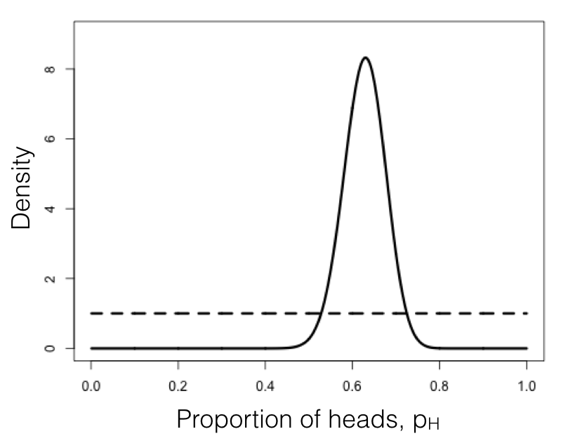
More data: lizard flipping (Harmon, Ch. 2)

Flip a lizard 100 times: observe 63 heads, 37 tails.
Two-sided binomial test of $H_0$: $f = 0.5$ gives $p = 0.006$, so we reject: the lizard is unfair.
But what is $f$? Likelihood: $$L(f|D) = f^{63}(1-f)^{37}$$
Maximum likelihood estimate: $\hat{f} = 63/100 = 0.63$.
Same idea as the coin, just with more data the likelihood is much more sharply peaked.

Fitting statistical models to data

Broadly, parameter estimation is more informative than test-statistics (i.e., $p$-values).
- Rejecting null hypotheses is rarely interesting in biology: the null is often obviously false.
Recall that the likelihood is: $$L(H|D) = P(D|H)$$
In an ML framework, the hypothesis with the highest probability of having generated the data is preferred.
ML will not always return accurate parameter estimates, even when the data is generated under the actual model.
- As with all estimators, ML improves with more data.

Likelihood Ratio Test

Can only compare two nested models: one must be a special case of the other.
Test statistic: $\Delta = 2(\ln L_1 - \ln L_0)$, where $L_1$ is the more complex model.
Under the null, $\Delta \sim \chi^2_k$ where $k$ is the difference in number of parameters.
Limitations:
- Results can depend on order of tests.
- Cannot compare non-nested models.

Akaike Information Criterion (AIC)

AIC balances model fit against model complexity: $$\text{AIC} = 2k - 2\ln L$$ where $k$ is the number of estimated parameters.
AIC assumes that reality is more complex than any of our models: the goal is to identify the model that most efficiently captures the important patterns in the data.
Lower AIC is better.
For small sample sizes, use the corrected version: $$\text{AIC}_c = \text{AIC} + \frac{2k(k+1)}{n-k-1}$$ AIC$_c$ is recommended for general use over generic AIC.

AIC weights

AIC weights provide a more interpretable way to use AIC outputs.
For model $i$ in a set of $R$ candidate models: $$w_i = \frac{e^{-\Delta_i/2}}{\sum_{r=1}^{R} e^{-\Delta_r/2}}$$ where $\Delta_i = \text{AIC}_i - \text{AIC}_{\min}$.
Can be interpreted as an estimate of the probability that model $i$ is the best model in the set.
Modern phylogenetic software frequently calculates AIC for model selection (e.g., ModelFinder in IQ-TREE).

Worked example: choosing a substitution model

A typical alignment fit by maximum likelihood under four nucleotide models. More-parameterised models fit better, but do they fit enough better? Here $k$ counts substitution-model free parameters; branch lengths are separate.

Model	$k$	$\ln L$	AIC	$\Delta$AIC	weight $w_i$
JC	0	$-2100.0$	4200.0	33.0	$\approx 0$
K80	1	$-2085.0$	4172.0	5.0	0.057
HKY	4	$-2079.5$	4167.0	0.0	0.690
GTR	8	$-2076.5$	4169.0	2.0	0.254

HKY wins the AIC trade-off. GTR's extra 3 lnL units of flexibility cost 4 extra parameters; HKY beats it by 2 AIC units.

Weights are graded. Read as "HKY 69%, GTR 25%, K80 6%, JC effectively 0%": the data's relative support among these four.

LRT agrees, where it can. JC$\to$K80: $\Delta = 30$ on $\chi^2_1$ ($p \ll 0.001$). K80$\to$HKY: $\Delta = 11$ on $\chi^2_3$ ($p = 0.012$). HKY$\to$GTR: $\Delta = 6$ on $\chi^2_4$ ($p = 0.20$). Keep HKY.

This is what IQ-TREE's ModelFinder and jModelTest do automatically, across many more models.

Bayes Factors

From posterior distributions, models can be compared using Bayes Factors: $$B_{12} = \frac{P(D|H_1)}{P(D|H_2)}$$
Bayes Factors are ratios of marginal likelihoods $P(D|H)$: the probability of the data averaged over all parameter values, weighted by the prior.
Unlike ML, this integrates over the full parameter space rather than evaluating only at the best-fit point.
Tends to favour simpler models than AIC. Assumes the true model is among those tested.

Prior (dotted) and posterior (solid) for the coin example. The marginal likelihood is the normalising constant of the posterior.

Harmon (2019) Phylogenetic Comparative Methods, Fig 2.3 (CC-BY-4.0).

Interpreting Bayes Factors

Kass & Raftery (1995) scale for $2\ln B_{12}$:

$2\ln B_{12}$	Evidence for $H_1$
0 to 2	Not worth more than a bare mention
2 to 6	Positive
6 to 10	Strong
> 10	Very strong

For nested models, $2\ln B_{12}$ is on the same scale as the LRT statistic.
Computing the marginal likelihood is hard. Common methods:
- Path sampling / stepping-stone
- Harmonic mean estimator (unreliable; avoid)
- Nested sampling

Kass & Raftery (1995) J Am Stat Assoc 90:773–795.

Model selection: summary

Method	Compares	Key assumption
Likelihood Ratio Test	Nested models only	Null model is true
AIC / AIC$_c$	Any models	Truth is more complex than any model
Bayes Factors	Any models	True model is among candidates

AIC and Bayes Factors can disagree: Bayes Factors may prefer a simpler model.
All methods assume good data and correctly specified candidate models.
Next lecture: we apply these tools to comparative trait data.