Darwin's Computer
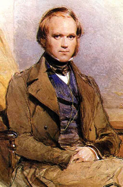

Detail from the only illustration in the Origin of Species (Darwin, 1859)
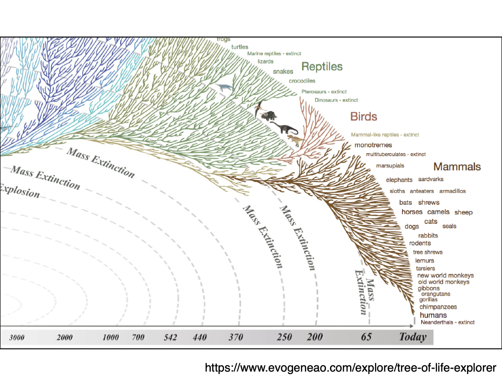
Descent with modification in populations
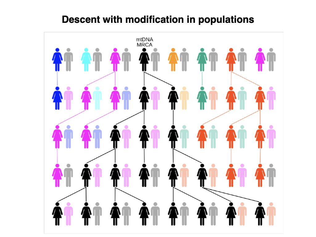
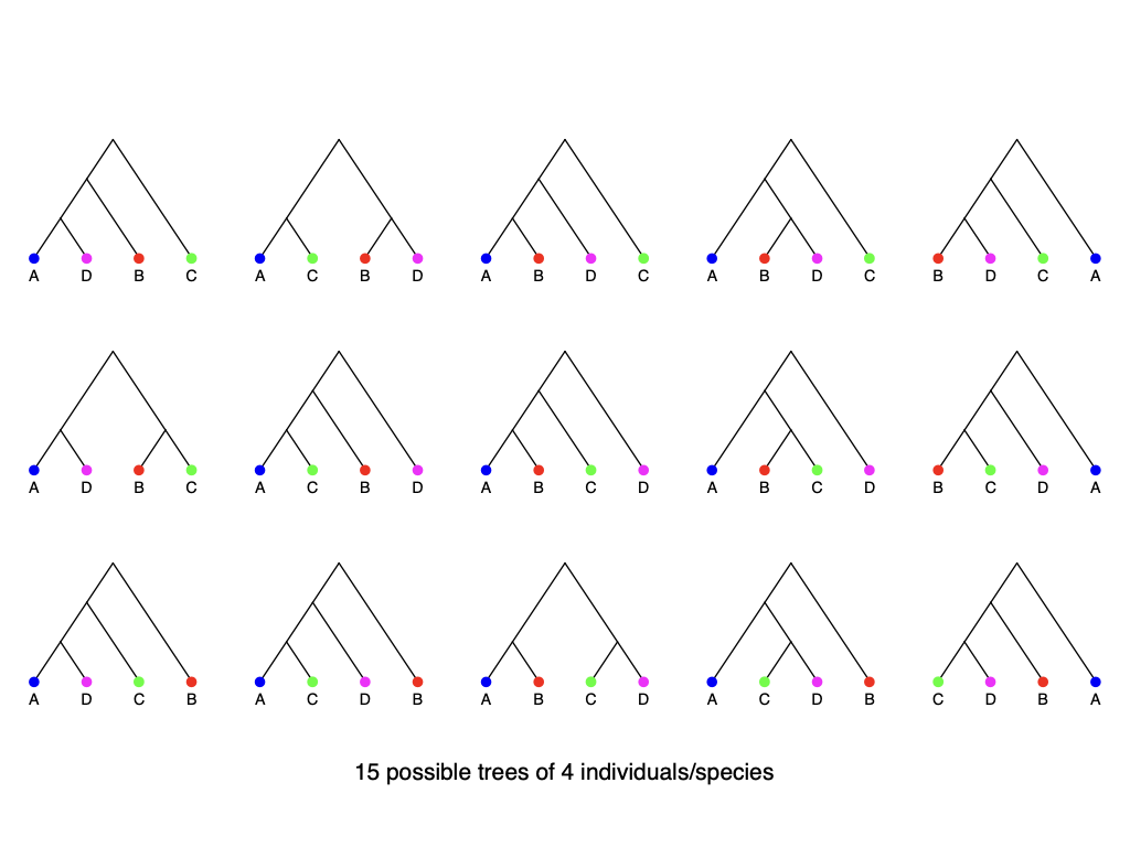
15 possible trees of 4 individuals/species
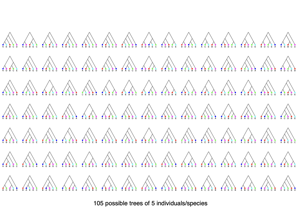
105 possible trees of 5 individuals/species
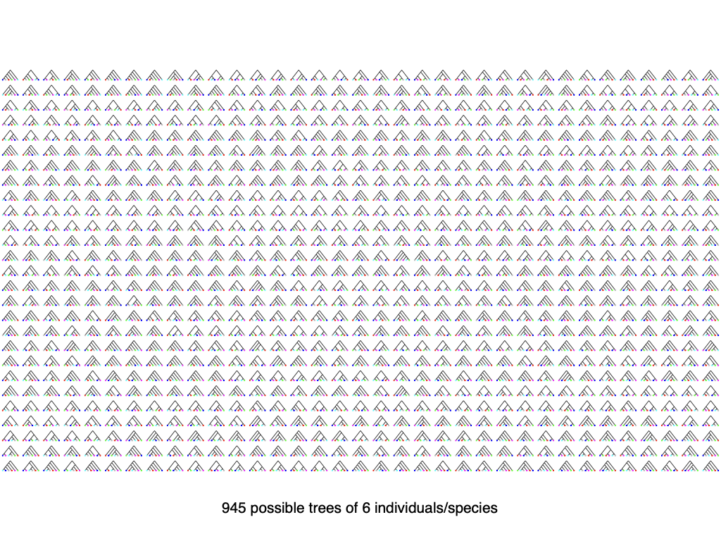
945 possible trees of 6 individuals/species
How many trees are there?
| $n$ | # rooted trees | |
| 4 | 15 | enumerable by hand |
| 5 | 105 | enumerable by hand on a rainy day |
| 6 | 945 | enumerable by computer |
| 7 | 10395 | still searchable very quickly on computer |
| 8 | 135135 | about the number of hairs on your head |
| 9 | 2027025 | greater than the population of Auckland |
| 10 | 34459425 | $\approx$ upper limit for exhaustive search |
| 20 | $8.2 \times 10^{21}$ | $\approx$ upper limit of branch-and-bound searching |
| 48 | $2.99 \times 10^{72}$ | $\approx 10^{22}$ times the number of atoms in the Earth |
| 136 | $5.69 \times 10^{269}$ | number of trees to choose from in the “Out of Africa” data (Vigilant et al. 1991) |
Computing Darwin's Tree of Life
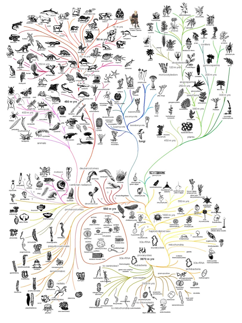
Bayesian reconstruction of phylogenetic trees
Yang & Rannala (1997), Mau, Newton & Larget (1998)
What we really want is the probability of the tree given the data.
We can compute that from the likelihood using Bayes Theorem:
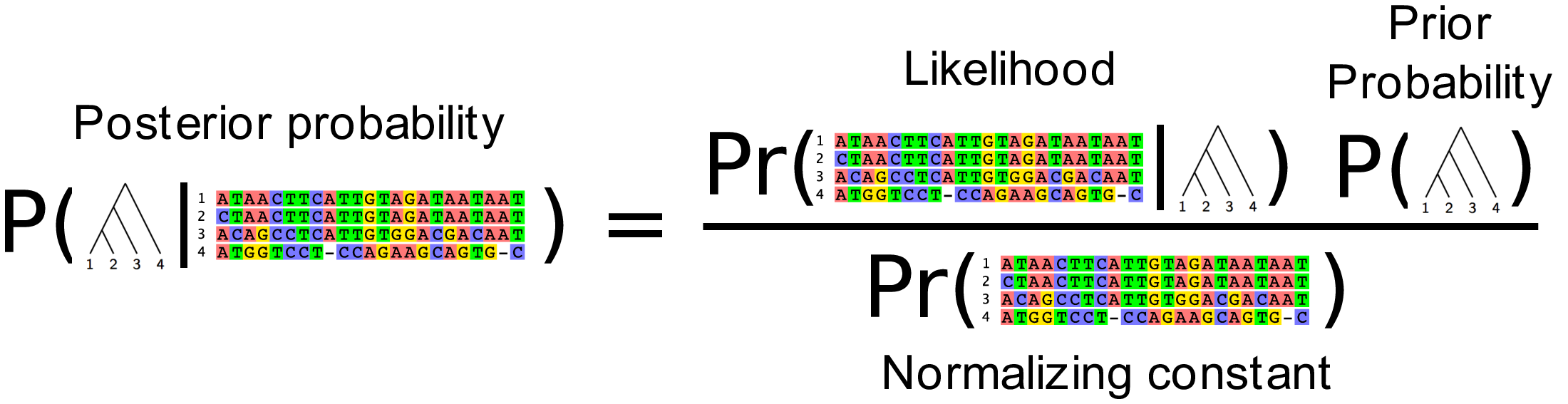
This is known as the Posterior probability of the tree. Using the Markov chain Monte Carlo algorithm we can produce a sample of trees that have high posterior probability.
Today is the overview. Every term here, prior, likelihood, posterior and MCMC, is unpacked from first principles in the next lecture.
The posterior distribution on Darwin's Finches
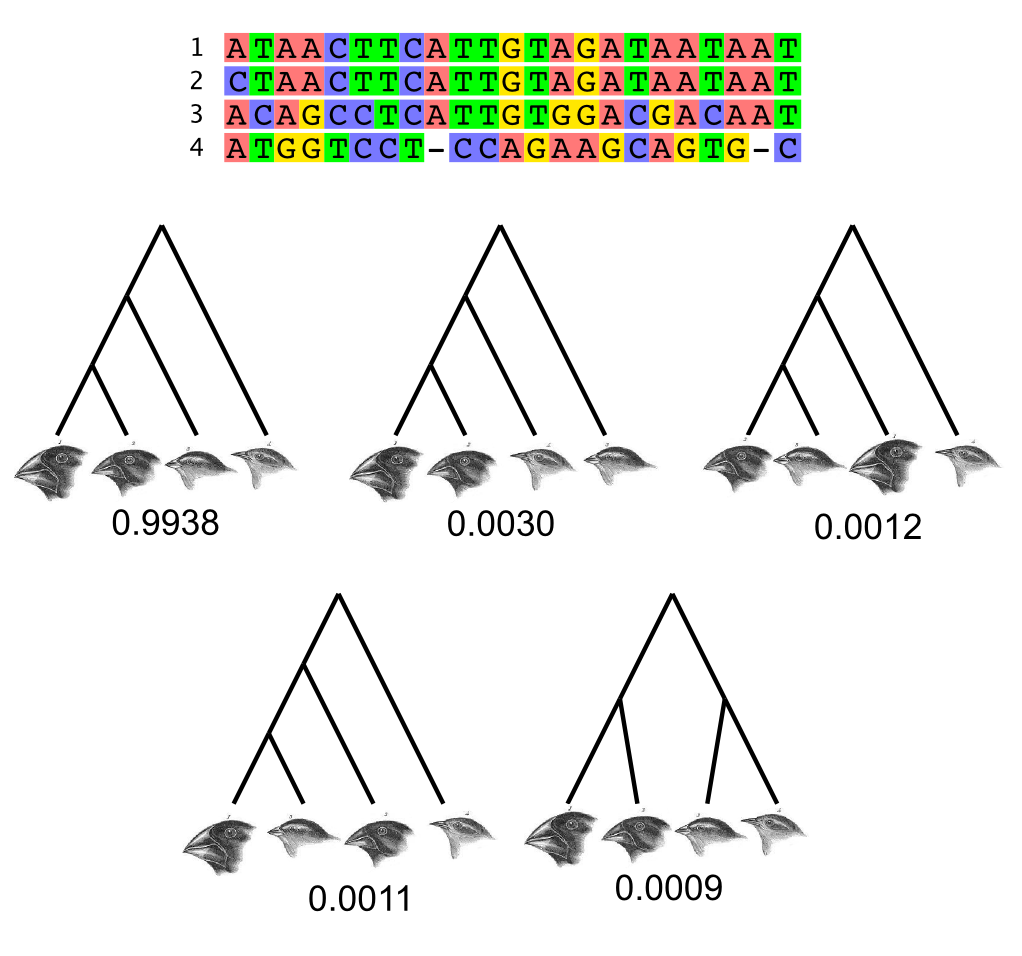
This posterior probability distribution was computed using Markov chain Monte Carlo implemented in the BEAST software package (Drummond et al, 2012).
The posterior distribution of larger trees
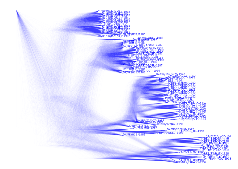
Elaborations of the phylogenetic model
Basic model: (posterior proportional to likelihood × prior)
$$P(\color{red}{g}|D) \propto \Pr(D|\color{red}{g}) \; P(\color{red}{g})$$Substitution model:
$$P(\color{red}{g},\color{#b8860b}{Q}|D) \propto \Pr(D|\color{red}{g},\color{#b8860b}{Q}) \; P(\color{red}{g}) \; \color{#b8860b}{P(Q)}$$Substitution model and tree branching process prior:
$$P(\color{red}{g},\color{#b8860b}{Q},\color{blue}{\Theta}|D) \propto \Pr(D|\color{red}{g},\color{#b8860b}{Q}) \; P(\color{red}{g}|\color{blue}{\Theta}) \; \color{#b8860b}{P(Q)} \; \color{blue}{P(\Theta)}$$$\color{red}{g}$ the tree · $\color{#b8860b}{Q}$ substitution model · $\color{blue}{\Theta}$ tree prior parameters · $D$ the sequence data
Elaborations of the model: Evolution is happening right now!
Modelling phylogenetic data sampled through time
Drummond and Rodrigo (2000), Drummond et al (2002)
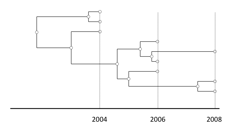
- Rapidly evolving microbes
- Ancient DNA
- Cancer
- Somatic evolution
- Languages
- et cetera
Sampling through time adds a clock rate $\color{darkgreen}{\mu}$, which converts the time tree $\color{red}{g}$ into the genetic distances the data actually record.
A calibrated phylogenetic inference
Origin of the HIV epidemic in the Americas, Gilbert et al (2007)
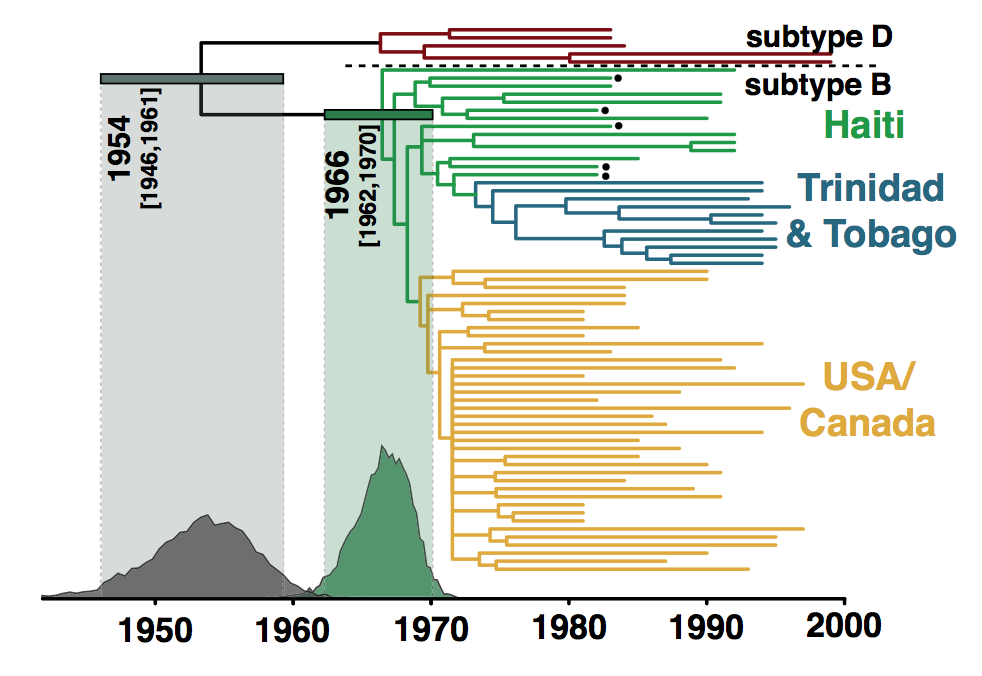
A phylogenetic reconstruction of samples of HIV-1 virus. Each tip represents a single infected individual from whom a blood sample has been taken.

Estimation of
- evolutionary trees
- divergence times
- evolutionary rates
- population history
- infectious disease parameters
- migration rates
- and more…
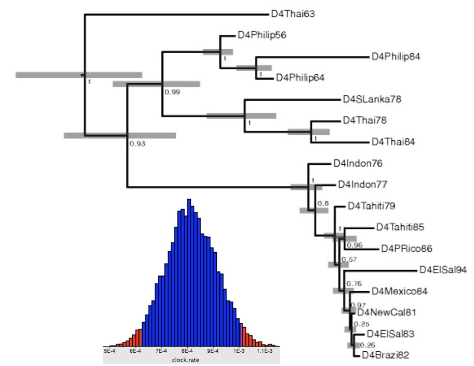
Also: Drummond & Rambaut, 2007; Drummond et al., 2012; Bouckaert et al., 2014; Suchard et al., 2018; Baele et al., Nat Methods, 2025
>42,000 scientific studies have cited the six BEAST papers,
>3,200 last year alone (2025)
Phylodynamics
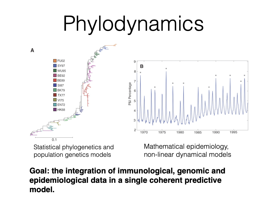
Statistical phylogenetics and
population genetics models
Mathematical epidemiology,
non-linear dynamical models
Goal: the integration of immunological, genomic and epidemiological data in a single coherent predictive model.
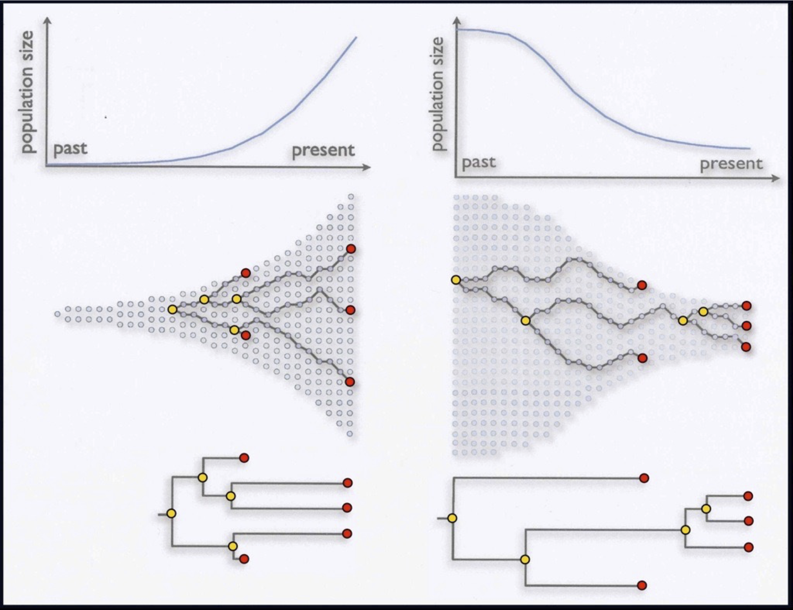
Coalescent theory: $P(g|\Theta)$
 $\Theta$
$g$
The same posterior as the previous slide. What is new is the identity of one factor: the coalescent supplies the tree prior $P(\color{red}{g}|\color{blue}{\Theta})$, and $\color{blue}{\Theta}$ becomes population size through time. (L10)
Trees inside trees
- Modelling diversity and divergence
- Central to understanding diverse areas including speciation genomics and host-symbiont co-evolution is building up a statistically rigorous model of the patterns of divergence and diversity spanning multiple species/hosts, multiple genes / gene families and multiple individuals per species/host.
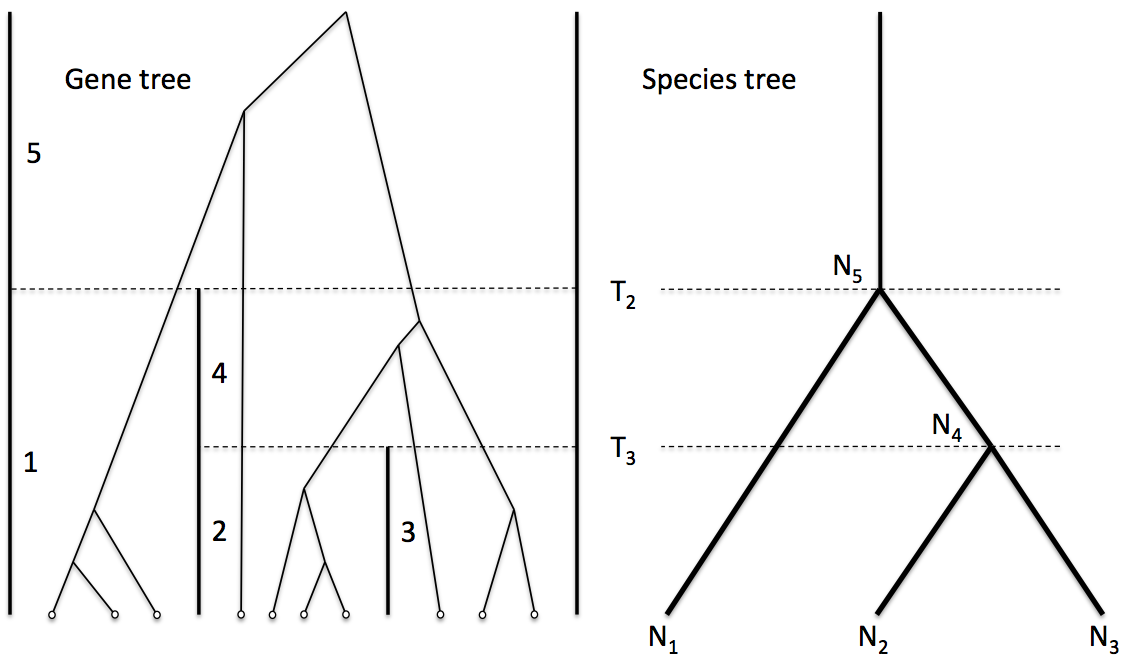
Now the tree prior on each gene tree $\color{red}{g_i}$ is itself supplied by a species tree $\color{purple}{S}$. (L11) The substitution model $\color{#b8860b}{Q}$ and clock rate $\color{darkgreen}{\mu}$ are suppressed here for simplicity; they remain part of the full model.
Phylogenies and the fossil record
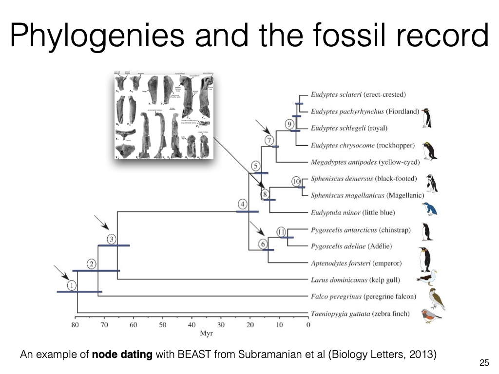
An example of node dating with BEAST from Subramanian et al (Biology Letters, 2013)
Perspectives
- Evolutionary biology has become a multidisciplinary analytical science, with major input from computer scientists, statisticians, mathematicians and physicists.
- Evolutionary biology is not just an historical science. Rapidly evolving natural systems, low-cost high-throughput sequencing and high-throughput automated experimental evolution platforms, all add up to the potential to close the loop between experimental and theoretical evolutionary biology.
- A common set of evolutionary modelling principles can inform us on diverse questions including human population history, the spread of viral epidemics and the age of fossils.
Where this module goes
Every equation today was a variation on one theme: a posterior over a tree, built from a likelihood and a tree prior. The rest of the module fills in that pattern.
- L8 Bayesian phylogenetic inference
- What prior, likelihood and posterior actually mean, and how MCMC computes them.
- L9 Molecular clocks and dated phylogenies
- The clock rate $\color{darkgreen}{\mu}$: how a tree gets a time axis in years.
- L10 The coalescent and population history
- The tree prior $P(\color{red}{g}|\color{blue}{\Theta})$ when $\color{blue}{\Theta}$ is population size.
- L11 Gene trees and the multispecies coalescent
- Gene trees $\color{red}{g_i}$ inside a species tree $\color{purple}{S}$.
- L12 Birth-death models and macroevolution
- Where the species tree $\color{purple}{S}$ itself comes from: speciation and extinction.
Recommended Reading
- Chapter 1: Introduction