Is evolution repeatable?
"…evolution over long time scales is utterly unpredictable and quite unrepeatable." (S. J. Gould, 1989)
What the math is for
By the end of these two lectures, you'll be able to read this sentence:
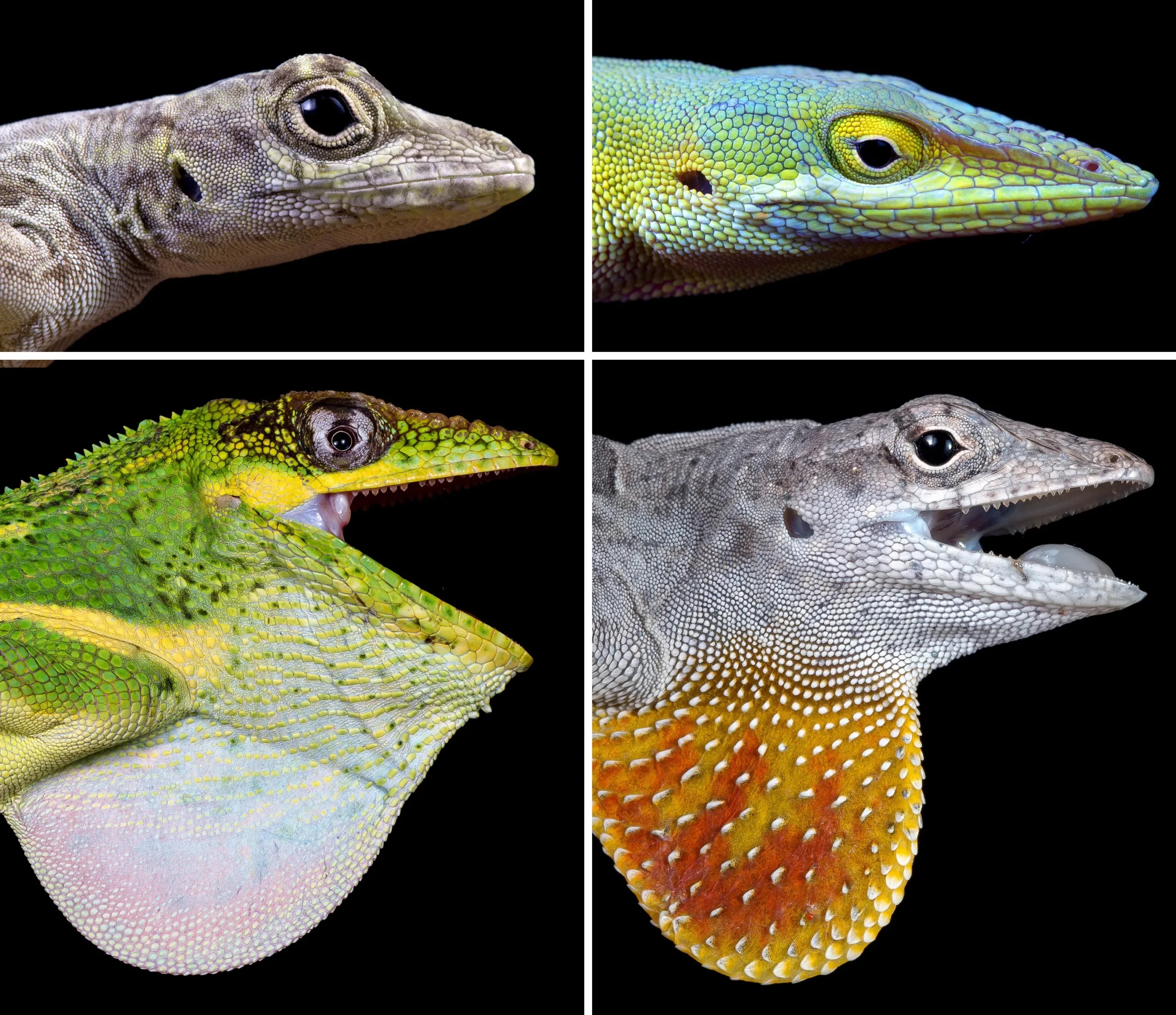
In English: four islands, four independent evolutionary experiments, and the same handful of lizard "ecomorphs" comes out each time. Within an adaptive radiation, convergence beats contingency.
Gould's argument was about deep-time evolution (replaying the whole history of life). An adaptive radiation unfolds over tens of millions of years in one ecological setting; it is the easier version of his question, and even here it took a lot of math to see the answer.
But first, a deeper problem stands in the way:
Are species independent data points?
No. Most of today's math is the price of fixing that.
Three tools we need to get from the question to the answer
- Handle shared ancestry. PIC, PGLS, the phylogenetic variance–covariance matrix $\mathbf{C}$. (This lecture.)
- Fit models with multiple adaptive peaks. Multivariate Ornstein–Uhlenbeck on the tree. (Next lecture.)
- Decide between models. $\mathrm{AIC}_c$ on a stepwise search. (Last lecture, used again here.)
Each tool plays a specific role when we return to the lizards at the end.
What are comparative methods?
- Comparing traits across species, often looking for correlations or causal relationships.
- e.g., two phenotypes across multiple species
- e.g., a phenotype against environment
- Bridging microevolutionary processes (genetic drift, selection) with macroevolutionary patterns across the tree of life (Harmon, Ch. 1).
- The field crystallised in the 1980s when Felsenstein (1985) showed that ignoring phylogenetic relatedness can lead to highly misleading conclusions.
- Synthesised by Harvey & Pagel (1991) and now a core tool in evolutionary biology.
Adaptive radiations: poster children of PCMs
- Rapid diversification, often without a fossil record.
- PCMs reconstruct evolutionary processes from extant species using a phylogeny.
- Did some clades evolve faster? Which traits co-evolve? Does an island habitat drive the radiation?
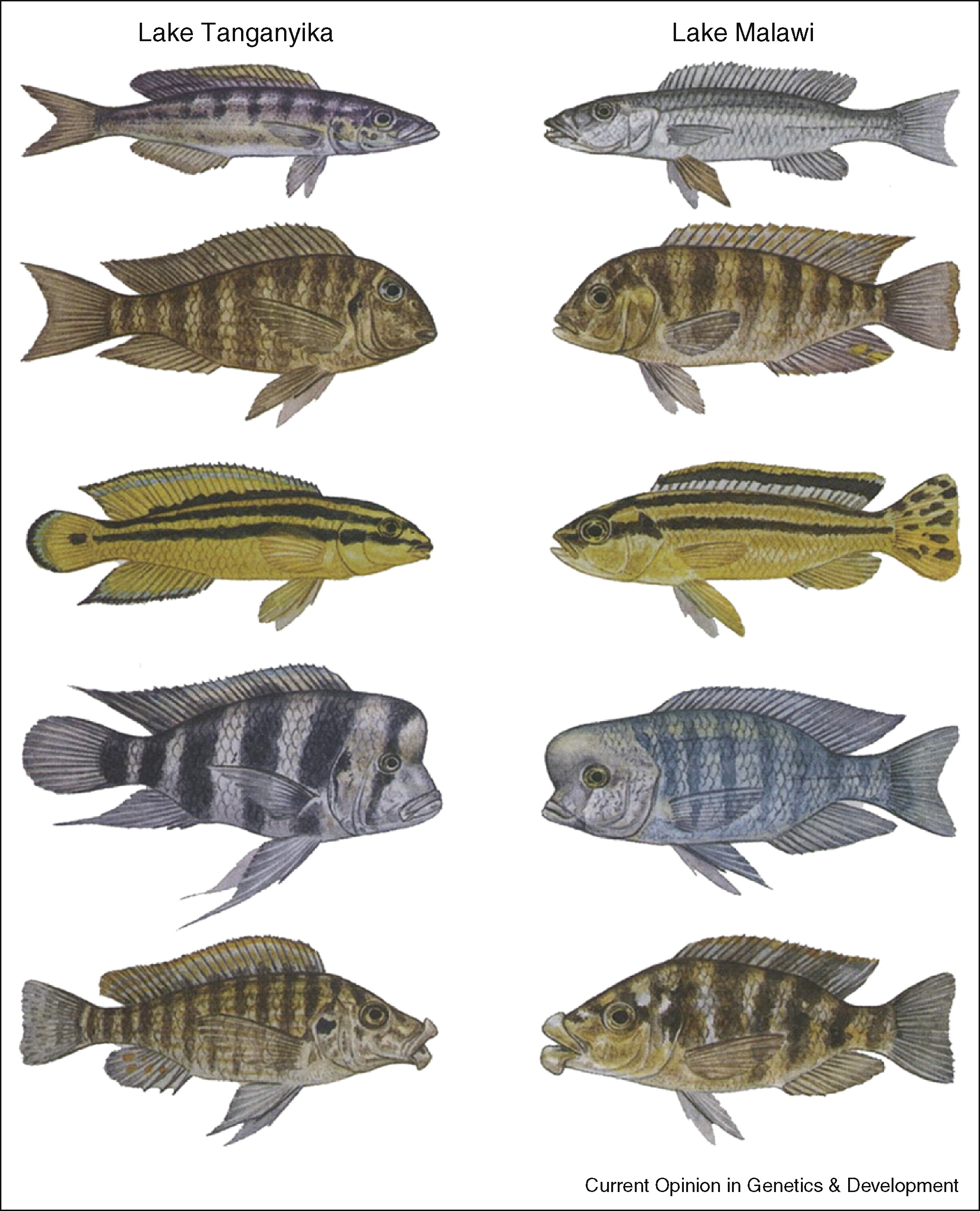
Cichlids: Kuraku & Meyer (2008) Curr Opin Genet Dev 18:551–558, Fig 4.
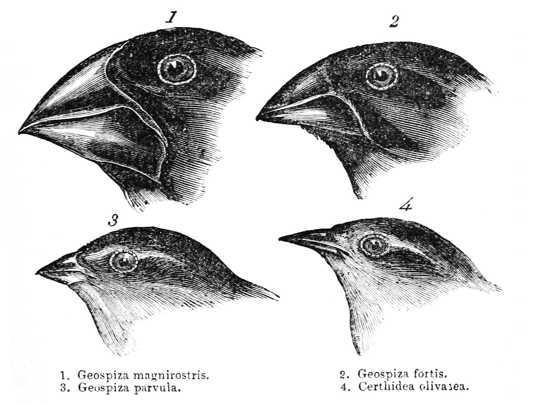
Finches: John Gould, The Zoology of the Voyage of H.M.S. Beagle (1845), public domain.
Two possible phylogenies for 8 species
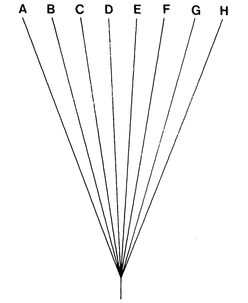
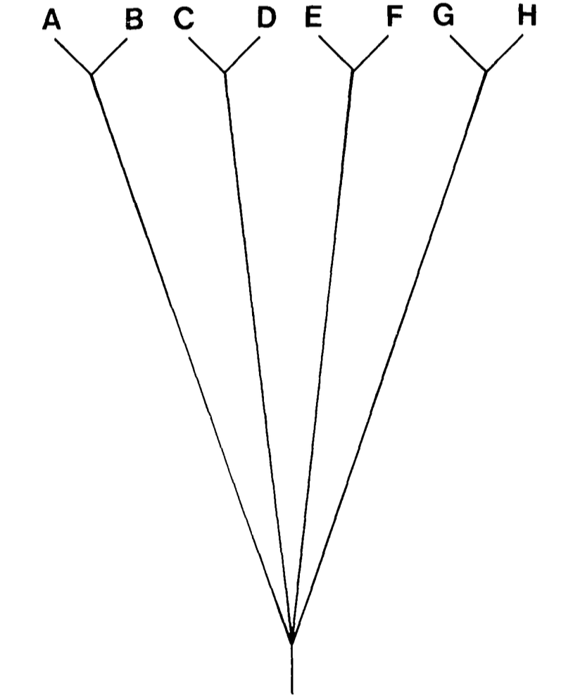
The problem of shared ancestry
- Consider 8 taxa: they may seem like 8 independent samples.
- But if they fall into two clades of 4, they are more like 4 independent samples.
- Treating them as independent can be misleading:
- Significance tests are more likely to report significance with 8 points than 4.
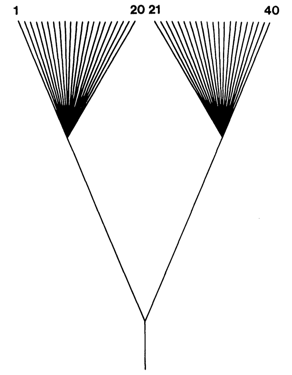
- Worst case: two deep lineages, each with many species.
- Sample all you want: you effectively have two data points, not 40.
- It doesn't matter which species you selected within each lineage.
The worst case
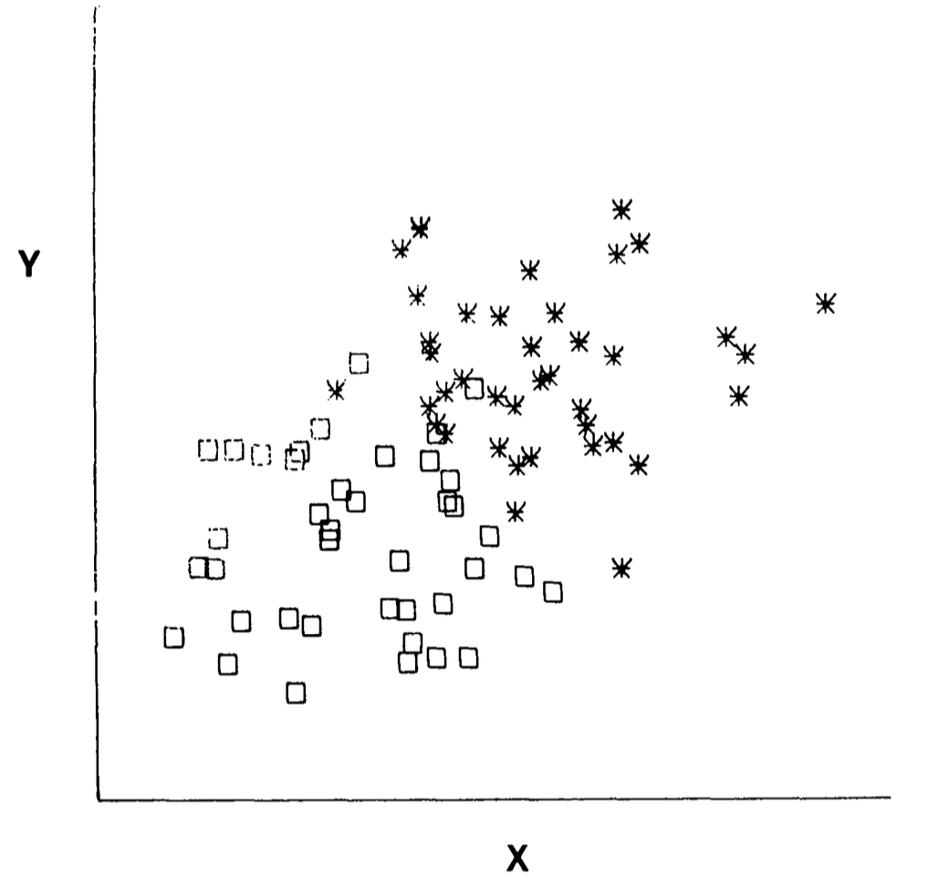
An apparent correlation...
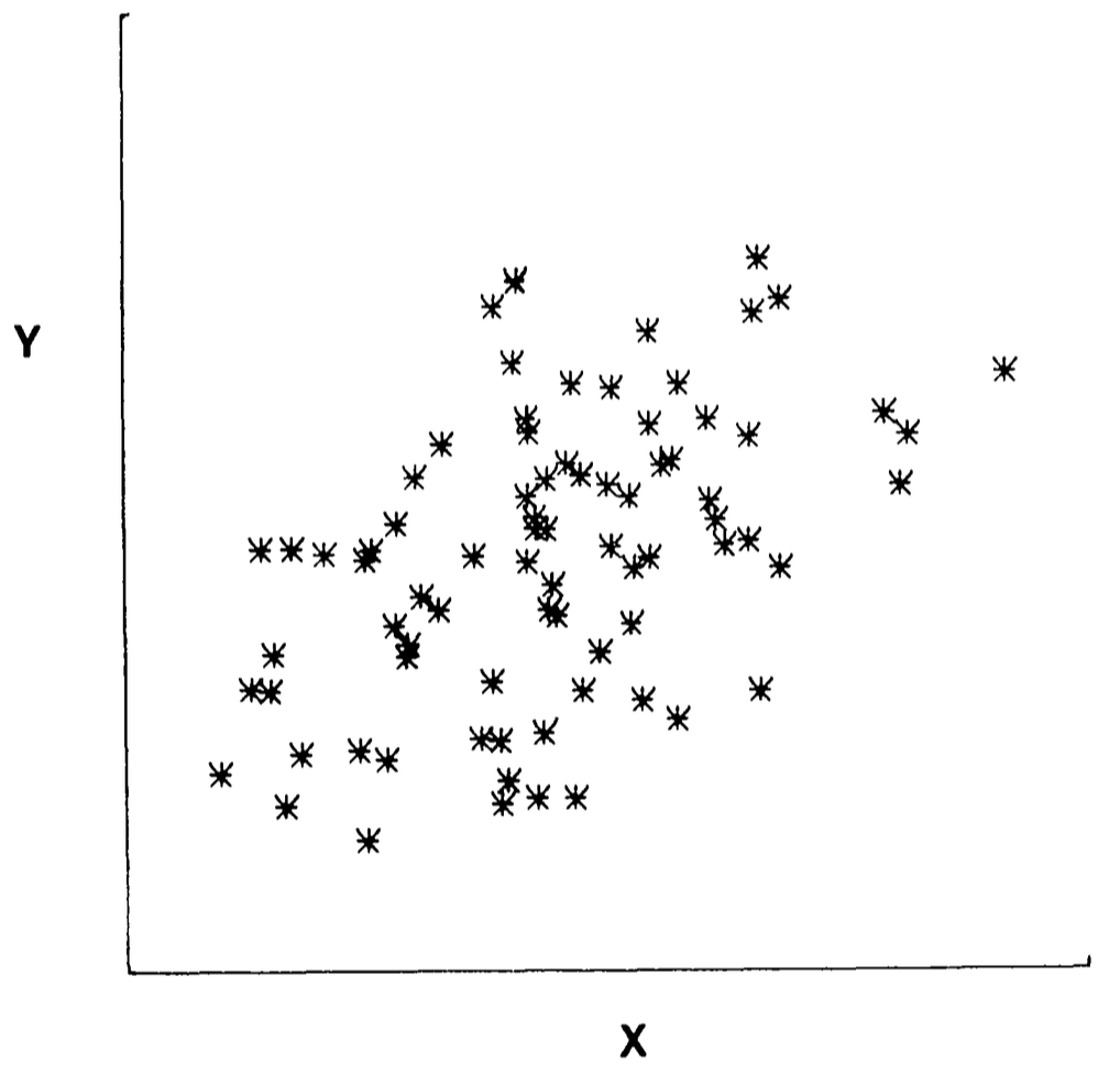
...is illusory
Try it yourself: the correlation illusion
Two clades, no real correlation.
Within each clade, $x$ and $y$ are independent. Only the clade means differ.
Tree shape: two star clades joined at a deep root (Felsenstein's worst case). Within each clade the $n$ tips are independent draws around the clade centre; the only real signal is the contrast between the two clade means.
Increase $d$, hold $\sigma$ small: $p$ shrinks fast. But the "signal" is really just 1 between-clade contrast.
Felsenstein's Phylogenetically Independent Contrasts
- Joseph Felsenstein (1985) introduced Phylogenetically Independent Contrasts (PIC) to address non-independence.
- The key insight: species on a shared phylogeny are not necessarily independent, so we must account for phylogeny in our comparative methods.
- This is always a risk except when:
"characters respond essentially instantaneously to natural selection in the current environment, so that phylogenetic inertia is essentially absent." (Felsenstein 1985)
A quick model: Brownian motion
- To handle the phylogenetic dependence, PIC assumes traits evolve by Brownian motion (BM).
- BM is a random walk in continuous time. After time $t$, starting at $X(0)$: $$X(t) \sim N\!\left(X(0),\; \sigma^2 t\right)$$
- Key properties:
- No directional trend: the expected value stays at $X(0)$.
- Variance grows linearly with time: long branches accumulate more change.
- The single rate parameter $\sigma^2$ governs how fast the trait changes.
- Why this works for PIC: differences between sister taxa under BM are independent draws from a normal distribution. We will return to BM in depth next lecture.
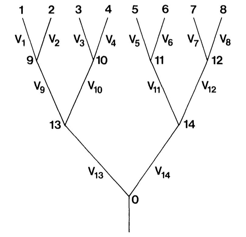
How PIC works
- Under BM, pairs of sister taxa provide independent samples of evolutionary change.
- Algorithm:
- Take a pair of sister tips and calculate a contrast (difference in trait values).
- Standardise by dividing by the square root of the sum of their branch lengths.
- Prune those tips, replace with a new tip at their ancestor with an estimated trait value, and adjust its branch length.
- Repeat until no more contrasts can be calculated.
- Standardised contrast for tips $i, j$ with branch lengths $v_i, v_j$: $$c_{ij} = \frac{X_i - X_j}{\sqrt{v_i + v_j}} \sim N(0, \sigma^2)$$
- The resulting contrasts are independent and can be used in standard statistical tests.
Try it yourself: step through PIC
Independent contrasts on a tree
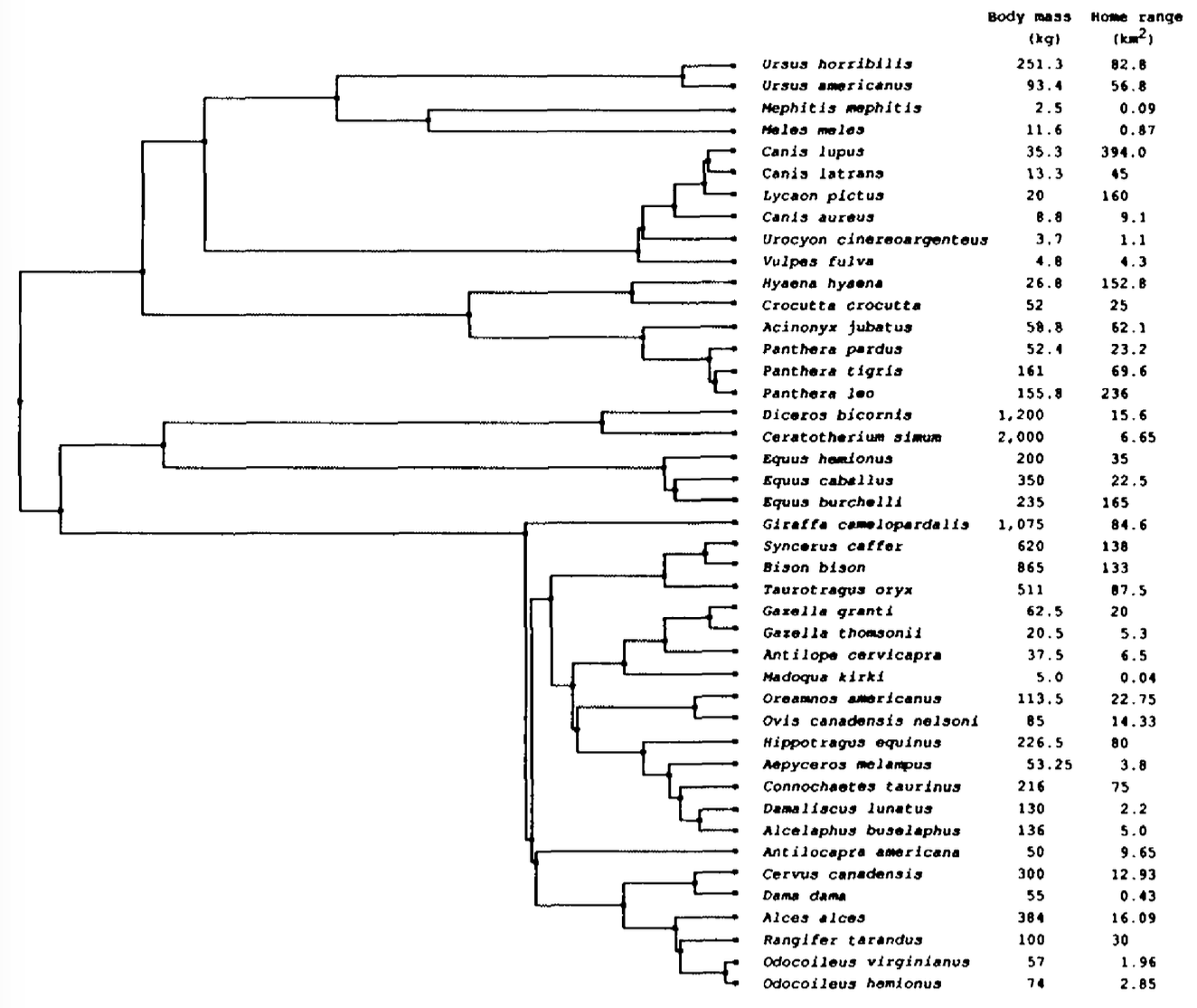
A real comparative dataset
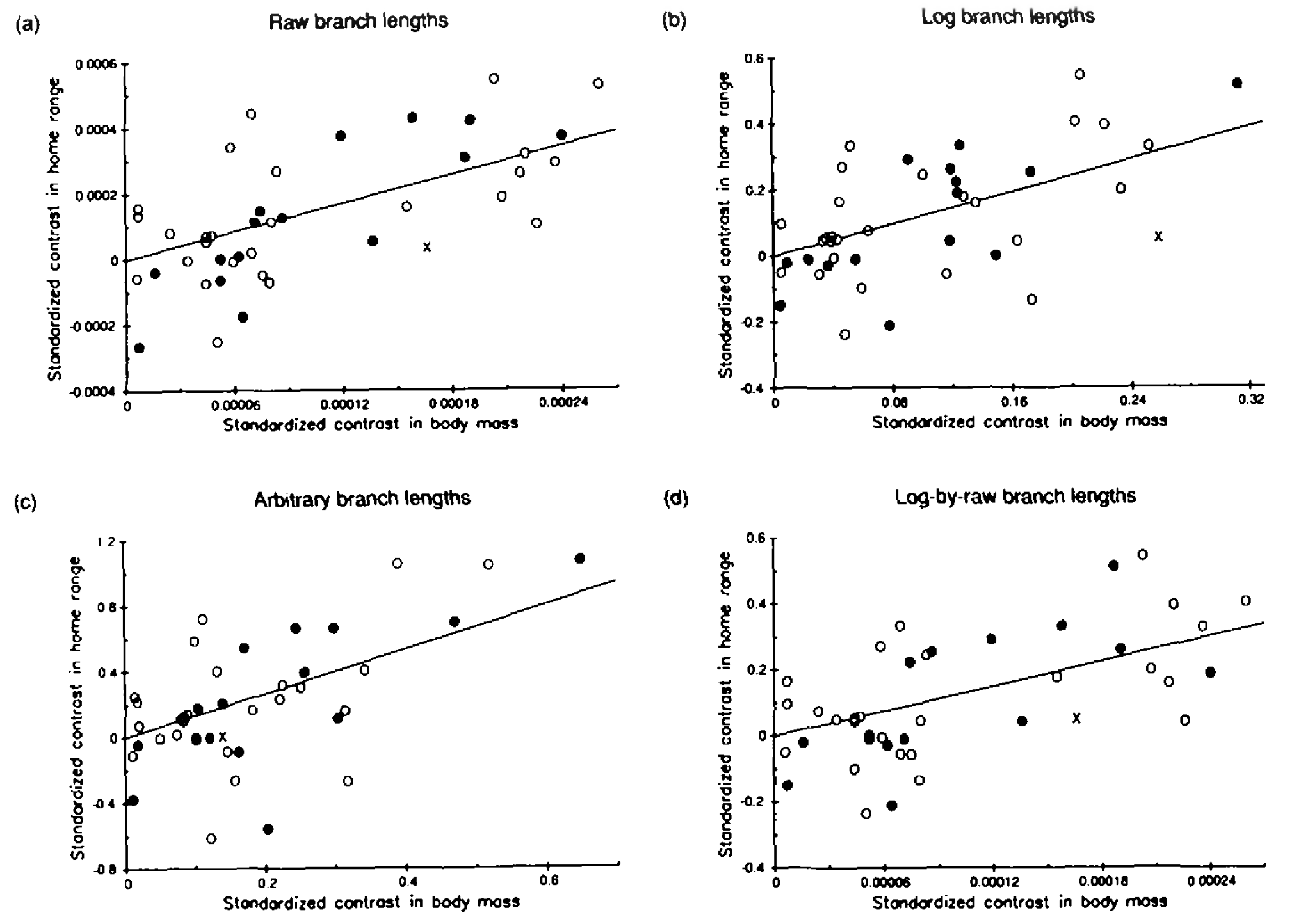
PIC on real data
From PIC to PGLS
Multivariate Brownian motion (Harmon, Ch. 5)
The phylogenetic variance–covariance matrix $\mathbf{C}$
$\mathbf{C}$: shared root-to-MRCA path
A&B share 2; A&C share 1; D shares 0 with anyone.
Inverse $\mathbf{C}^{-1}$
Negative off-diagonals down-weight related species.
Multivariate Brownian motion
- PIC handles one trait at a time. What if two traits evolve together?
- Multivariate BM: $r$ traits with a rate matrix $\mathbf{R}$:
$$\mathbf{R} = \begin{pmatrix} \sigma_x^2 & \sigma_{xy} \\ \sigma_{xy} & \sigma_y^2 \end{pmatrix}$$
- Diagonal: per-trait evolutionary rates.
- Off-diagonal: evolutionary covariance $\sigma_{xy}$ between traits.
- The joint distribution of all tip values pairs $\mathbf{R}$ (how traits co-evolve) with $\mathbf{C}$ (how taxa share ancestry). For one trait at a time, the tip variance is $\sigma^2 \cdot \mathbf{C}$. For two traits, the cross-trait covariance is $\sigma_{xy} \cdot \mathbf{C}$, same shape, scaled.
- $\sigma_{xy} \ne 0$ means the traits have a real evolutionary tendency to change together, beyond the patterns shared ancestry alone produces.
How do we actually use $\mathbf{V}$?
- The stacked tip vector $\mathbf{d} = (X_A, \ldots, X_n, Y_A, \ldots, Y_n)^\top$ has a closed-form distribution: $$\mathbf{d} \sim \mathrm{MVN}(\boldsymbol{0},\; \mathbf{V})$$ so we can write down the likelihood $L(\mathbf{R}, \mathrm{tree} \mid \mathbf{d})$ directly.
- Estimate the rate matrix. Given a tree and the observed tips, find the $\mathbf{R}$ (the three numbers $\sigma_x^2, \sigma_y^2, \sigma_{xy}$) that maximises this likelihood. The MLE of $\sigma_{xy}$ is the estimate of evolutionary covariance.
- Test for evolutionary correlation. Compare two nested models with a likelihood-ratio test:
- $H_0$: $\sigma_{xy} = 0$ (independent evolution).
- $H_1$: $\sigma_{xy}$ free.
- Simulate. Sample from $\mathrm{MVN}(\boldsymbol{0},\mathbf{V})$ to generate synthetic data under a null, or to check a fitted model.
- Regress $Y$ on $X$. Take one trait as response, the other as predictor: this is PGLS (next slide). Unlike the symmetric covariance above, regression is asymmetric: here $X$ predicts $Y$. It uses just $\mathbf{C}$, not the full $\mathbf{V}$.
Evolutionary correlation vs. spurious correlation
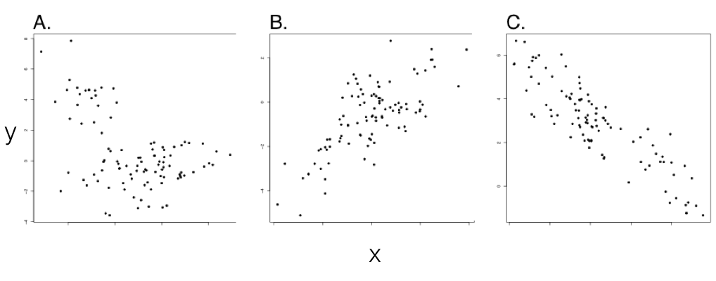
Each point is one species. $x$-axis: tip value of trait $X$. $y$-axis: tip value of trait $Y$.
$n = 100$ species simulated under multivariate BM on a pure-birth tree, with $\sigma_x^2 = \sigma_y^2 = 1$.
No evolutionary covariance, but clustering by clade can still produce apparent patterns: spurious.
Genuine positive co-evolution: large $X$ predicts large $Y$.
Genuine negative co-evolution: large $X$ predicts small $Y$.
Phylogenetic GLS (PGLS): related species count for less
Same residuals, measured two ways:
OLS minimises the plain sum of squares: $$\textstyle\sum_i (y_i - \hat{y}_i)^2$$
PGLS measures them in the metric set by $\mathbf{C}^{-1}$: $$(\mathbf{y} - \mathbf{X}\boldsymbol{\beta})^\top \, \mathbf{C}^{-1} \, (\mathbf{y} - \mathbf{X}\boldsymbol{\beta})$$
Recall $\mathbf{C}^{-1}$ (two slides back)
The sister pair A, B got the big negative entry $-5/13$: shared ancestry, so they partly cancel.
D, related to no one, kept a clean $1/3$: it counts as one full independent sample.
PGLS: where the slope comes from
- Minimising that weighted sum of squares has a closed-form answer:
$$\hat{\boldsymbol{\beta}} = (\mathbf{X}^\top \mathbf{C}^{-1} \mathbf{X})^{-1}\, \mathbf{X}^\top \mathbf{C}^{-1} \mathbf{y}$$This is textbook generalised least squares: the same formula used whenever errors are correlated. Your software computes it; you never do it by hand. Phylogeny enters only through $\mathbf{C}$, the known covariance structure due to shared ancestry.
- $\mathbf{X}$ is the predictor (design) matrix: a column of 1s for the intercept and a column of the predictor values $x$ for the slope.
- Software defaults to this: caper::pgls, phylolm, nlme::gls.
A single-response regression needs only $\mathbf{C}$, not the full multi-trait $\mathbf{V}$ from the correlation slides.
A concrete phylogenetic regression
| sp | $x$ | $y$ |
|---|---|---|
| A | 1 | 2 |
| B | 2 | 5 |
| C | 3 | 8 |
| D | 7 | 10 |
Fit an intercept and a slope, with the phylogeny in the errors:
$$y = \beta_0 + \beta_1 x + \varepsilon, \qquad \varepsilon \sim \mathrm{MVN}(\mathbf{0},\, \sigma^2\mathbf{C}).$$Software solves the now $2\times2$ sandwich $\hat{\boldsymbol{\beta}} = (\mathbf{X}^\top\mathbf{C}^{-1}\mathbf{X})^{-1}\mathbf{X}^\top\mathbf{C}^{-1}\mathbf{y}$:
$\hat{\beta}_1 = \tfrac{4}{3} \approx 1.33$
$\hat{\beta}_0 \approx 1.84$
$\hat{\beta}_1 \approx 1.19$
$\hat{\beta}_0 \approx 2.37$
- Slope $\hat{\beta}_1$: each one-unit rise in $x$ goes with a ~1.33-unit rise in $y$, shared ancestry removed.
- Intercept $\hat{\beta}_0$: fitted $y$ at $x=0$. The line pivots through the phylogenetic centroid $(\bar{x}_w,\bar{y}_w) = (4,\,7.18)$.
OLS vs PGLS on real data
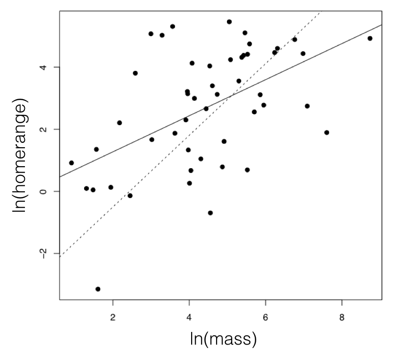
- Same data as Garland (1992), now fitted two ways.
- OLS slope ≈ 1.0. PGLS slope ≈ 0.5.
- OLS over-estimates the relationship by treating closely related species as independent samples.
- PGLS corrects this and is closer to the true evolutionary slope.
Try it yourself: OLS vs PGLS
Simulated BM on an 8-tip balanced tree.
Generate $(x,y)$ at the tips under multivariate BM with rate matrix $\mathbf{R}$.
PGLS computed via Felsenstein's contrasts (equivalent under BM).
Set $\sigma_{xy} \approx 0$, hit re-sample several times: OLS often shows a strong slope just from shared ancestry.
PCMs in the wild: three case studies
Common thread: each study would have given a misleading answer with naive (non-phylogenetic) analysis.
PIC / PGLS: assumptions and limitations
- Assume traits evolve by Brownian motion. How reasonable is this?
- Beyond-BM models (OU, early burst, $\lambda$) relax this. See next lecture.
- Assume the phylogeny is known without error (topology and branch lengths).
- For PGLS regression: assume the predictor is fixed, not evolving. Often violated for trait-vs-trait questions.
- Despite limitations, PIC/PGLS were foundational advances:
- Showed that ignoring phylogeny can lead to seriously misleading conclusions.
- Opened the field of phylogenetic comparative methods.
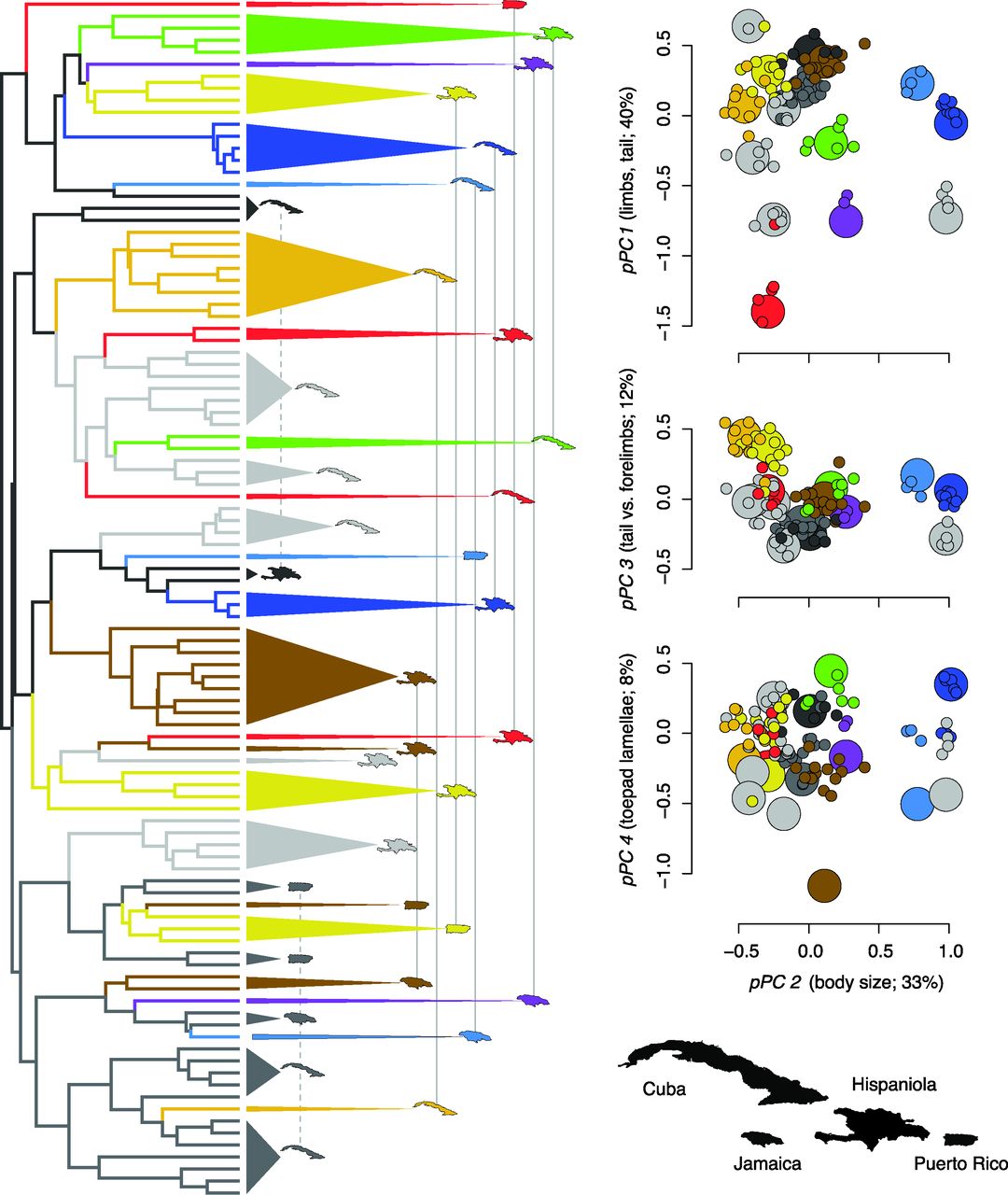
Example: convergence on the macroevolutionary landscape
Mahler, Ingram, Revell & Losos (2013) Science 341:292
A whole-fauna test of replicated radiation
- Setup. 100 of 119 Anolis species across Cuba, Hispaniola, Puerto Rico, and Jamaica. 11 ecomorphological traits $\to$ 4 phylogenetic PC axes. MCC tree from a BEAST analysis of mtDNA.
- Old story. Each island has the same handful of named ecomorphs (twig, grass-bush, trunk-crown…): convergence among matched species.
- New question. When you include the "unique" species too (~20% of the fauna), are entire island radiations still more similar than chance?
- Why we care. The paper combines two threads from this session: a multivariate, multi-peak trait model (this lecture) and stepwise AICc model comparison (last lecture).
The Hansen model: a multi-peak OU on the tree
- Each lineage evolves under an Ornstein–Uhlenbeck process: $$dX = \alpha(\theta - X)\,dt + \sigma\,dW$$ BM noise $\sigma^2$, pulled toward an optimum $\theta$ with strength $\alpha$. (We meet OU properly in the next lecture.)
- Multi-peak twist. Paint the branches of the tree with regimes. Each regime has its own $\theta_i$, an adaptive peak in trait space.
- Parameters: $\sigma^2$, $\alpha$, and $\theta_1,\ldots,\theta_{k'}$. With $m$ traits, each $\theta_i$ is an $m$-vector; this is the multivariate piece.
- Captures Simpson's "adaptive zones" mathematically: lineages that share a regime are pulled toward the same point on the landscape.
SURFACE: stepwise AICc on the landscape
- Problem. Where do the peak shifts go on the tree? How many peaks? Which shifts are convergent? Too many possibilities to enumerate.
- SURFACE (Ingram & Mahler 2013) is a two-phase stepwise AICc search, the same logic as L11 applied to the multi-peak OU model:
- Forward phase. Start from a single-peak OU. At each step, try placing a new shift on every branch; keep the placement that lowers AICc the most. Stop when nothing helps.
- Backward phase. Try collapsing every pair of peaks into a single shared peak (= convergence). Each collapse removes $m$ optimum parameters, so AICc can improve even though the log-likelihood cannot.
- Crucially, ecomorph labels are not used as input. Any convergence the method finds is data-driven.
- Parameter count for $k$ shifts and $k'$ distinct peaks: $\,k + (k'+2)\,m$. Forward phase has $k'=k$; backward phase drives $k' < k$.
The result: AICc picks a convergent landscape
| single-peak OU | 340.4 |
| BM / EB / time / lineage‑diversity (no peaks) | $\geq 279.3$ |
| non-convergent multipeak (forward phase only) | 162.6 |
- 29 peak shifts collapsed to 15 distinct peaks.
- 22 / 29 (76%) shifts are convergent.
- 7 / 8 convergent peaks span more than one island.
- Endemic "unique" peaks occur only on the two largest islands: an area effect.
And at scale: 9,963 birds, same logic

- Data. 9 morphological traits for 9,963 bird species ($>99\%$ of extant birds, all 233 families). $\to$ 4-D morphospace.
- Method. BAMM (reversible-jump Bayesian MCMC over trait-rate regimes) + random-forest niche prediction + Monte-Carlo tests against a phylogenetic null.
- Result. 91 family pairs reach the same region of morphospace from independent origins, typically in disjunct biogeographical realms: toucans (Neotropics) and hornbills (palaeotropics); antpittas and pittas; swifts and swallows.
- Same question, different methods. Mahler picks among competing OU models by $\mathrm{AIC}_c$. Pigot fits a Bayesian rate-shift model and tests convergence against a simulated null. Statistically comparing competing evolutionary hypotheses is genuinely hard, and methods continue to evolve.
Discussion
- Can you imagine a situation where "phylogenetic inertia is essentially absent"?
- How reasonable is the assumption that traits evolve by Brownian motion?
- You are studying the surface proteins of a human pathogen. The primary selective force is for them to look different from generation to generation. Is PIC appropriate here?
- In the OLS-vs-PGLS demo, when $\sigma_{xy}=0$ but you still see a non-zero OLS slope: where is that signal coming from?
- In Mahler et al., the convergent landscape beats a non-convergent multipeak model by $\Delta\mathrm{AIC}_c = 162.6$. The two models use the same shift placements, so what is the convergent model trading off to win, and why does AICc reward it?
Recommended Reading
- Chapter 8: Traits and Comparative Methods
- Chapters 1, 3, 5: macroevolutionary research, Brownian motion, multivariate BM
- Mahler, Ingram, Revell & Losos (2013). Exceptional convergence on the macroevolutionary landscape in island lizard radiations. Science 341:292.
- Pigot et al. (2020). Macroevolutionary convergence connects morphological form to ecological function in birds. Nat Ecol Evol 4:230.