Where we are going

• A gene tree is not just a record of who is related to whom. Its shape carries information about the population the sample came from.
• Part 1. The coalescent: where gene trees come from, and why the size of a population controls how deep its trees are.
• Part 2. Running the argument backwards: reading a population's history off the trees, and what that has revealed about humans and about epidemics.

In Lecture 8 the tree prior was an empty slot in the model. This lecture fills it.

The setting

Data: a small genetic sample from a large background population.

• We will never sequence the whole population, and we do not need to.
• The coalescent is a model of the ancestry of a sample, traced backwards in time until every lineage has met.
• It gives a probability distribution over trees, given a population history. That makes it exactly the kind of tree prior that Lecture 8 needed.
• Being a model of genealogies rather than of sequences, it assumes the sampled sites are evolving neutrally.

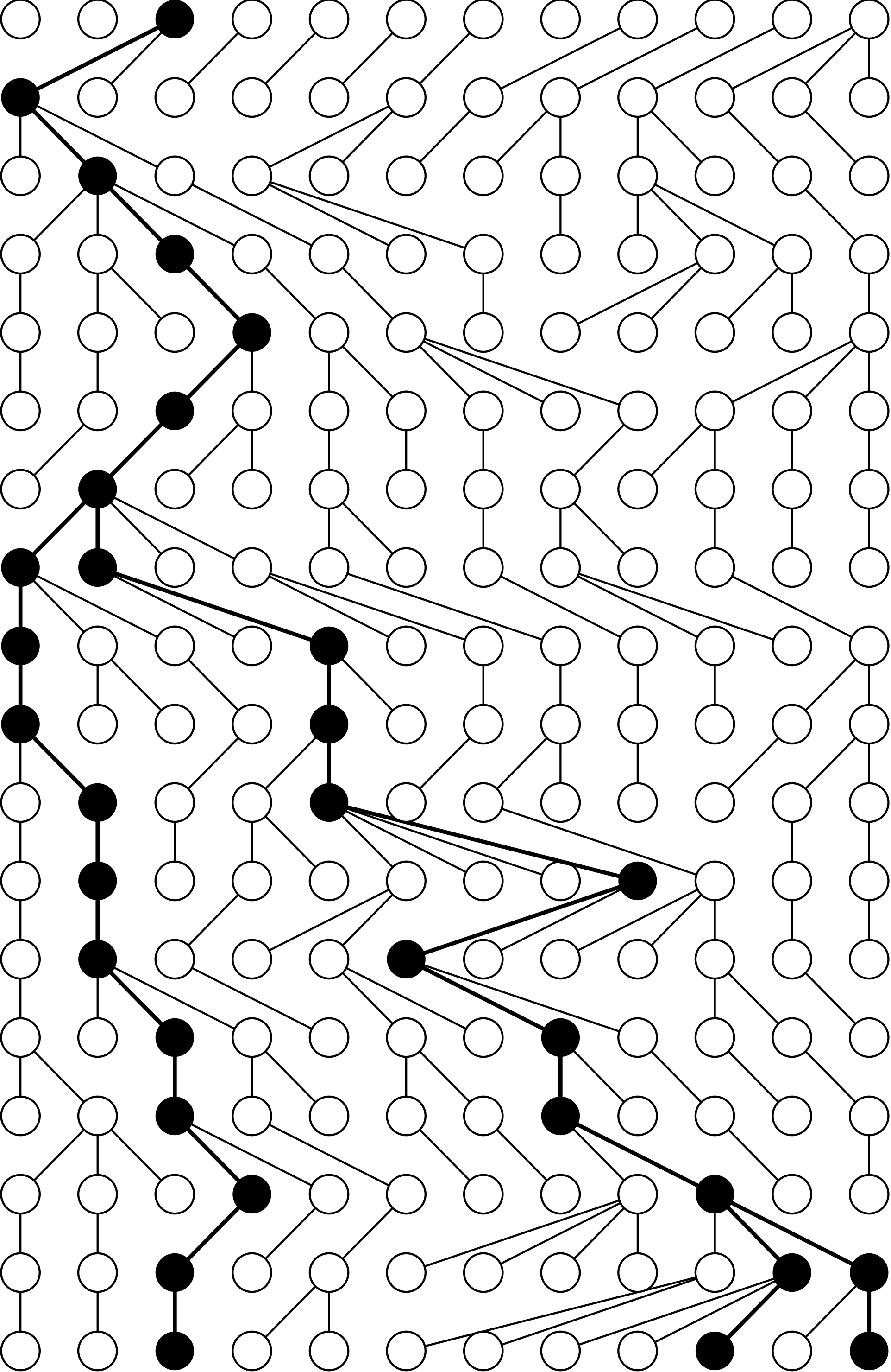
The Wright-Fisher population

Almost all of theoretical population genetics starts from one deliberately simple picture of a population:

• Constant size $N$.
• Discrete, non-overlapping generations.
• Complete mixing: every individual in one generation picks its parent at random from the generation before.

That last rule is the whole model. Everything else follows from it.

We will treat the population as haploid, which is the natural case for many pathogens and for mitochondrial DNA.

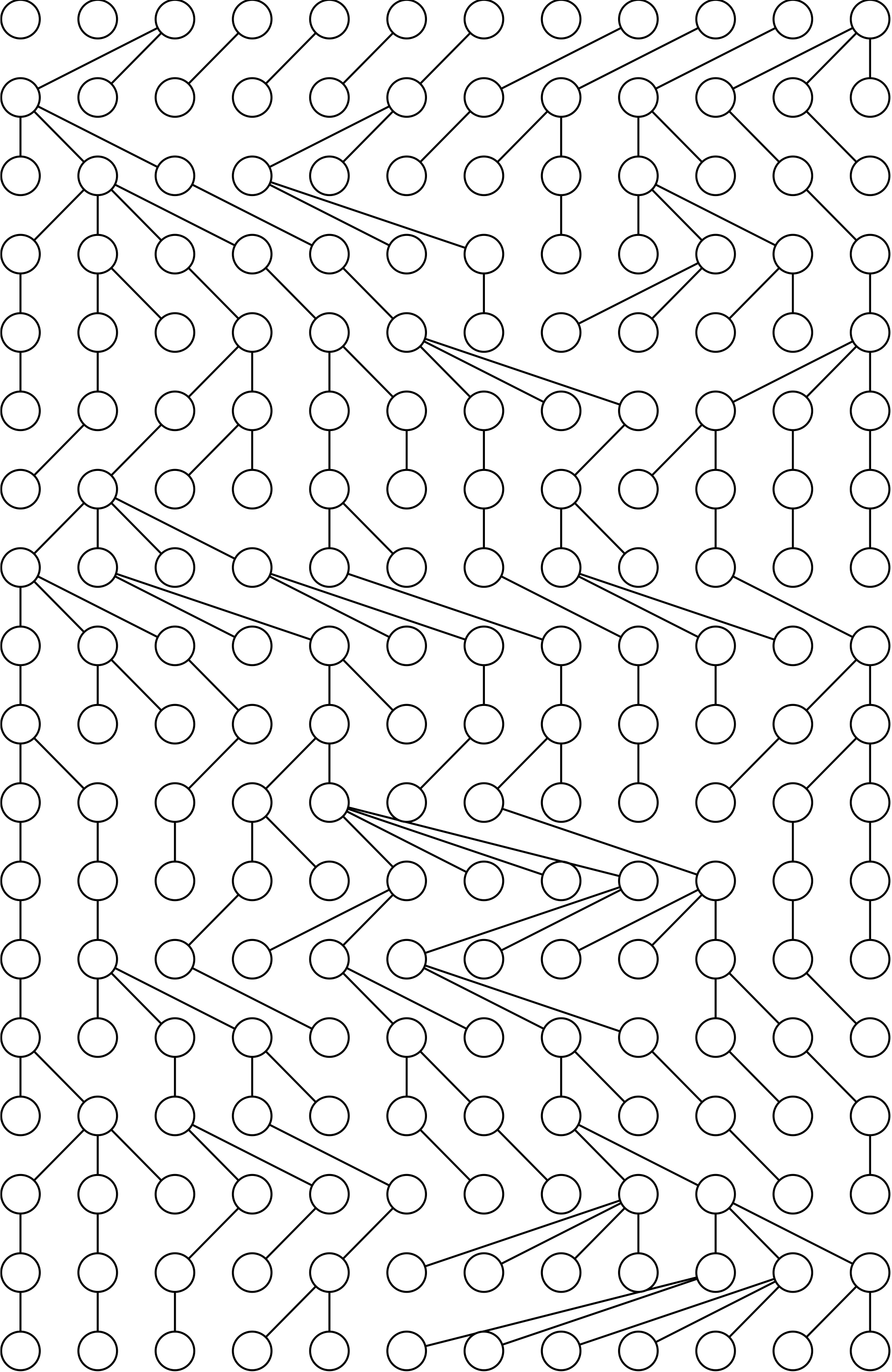
Try it yourself: tracing a sample back

The one rule that matters

• The waiting time is longer in a large population and shorter in a small one. This is the link between tree shape and population size, and it runs in both directions.
• With many lineages there are many pairs, so early coalescences come thick and fast. As lineages are used up, the waits get longer.
• Coalescent trees are therefore lopsided: crowded near the tips, with one very long branch pair at the root. Half the total depth of the tree is spent waiting for the last two lineages to meet.

From a population to a tree

Strip away everyone who left no descendants in the sample, and what remains is a tree:

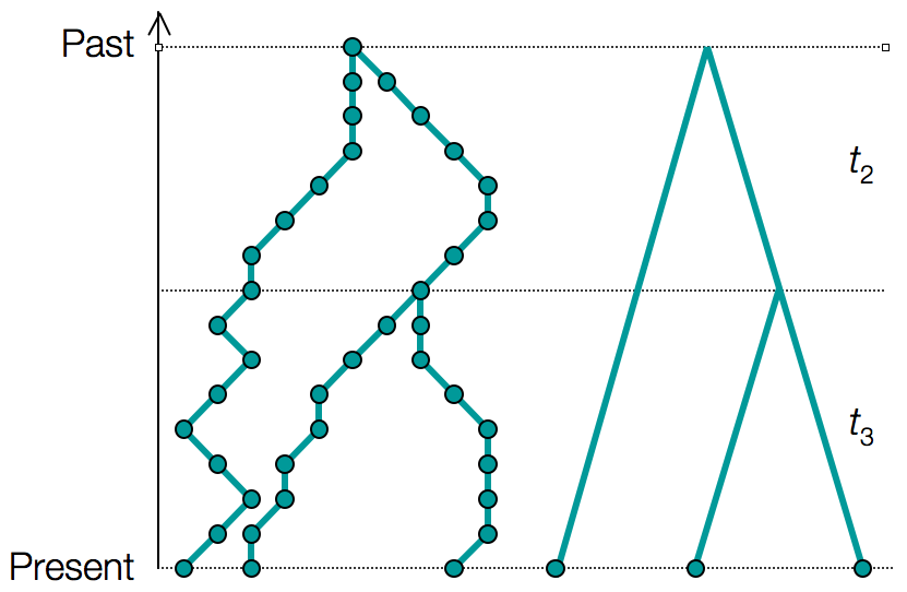
The coalescent gives the probability of any such tree, given the population history. In a Bayesian analysis that is precisely $P(T \mid \theta)$: the tree prior.

A changing population leaves a signature

If population size controls the waiting times, then a population whose size changed leaves trees of a characteristic shape:

Constant size

The familiar coalescent tree: crowded tips, long root branches.

A population that grew recently

Going backwards, the population shrinks, so coalescence speeds up in the past. Every lineage meets at almost the same time and the tree looks like a star, with long parallel tips.

A bottleneck

While the population is small, coalescence is very fast. Lineages pile into the bottleneck and the tree shows a burst of branching at that depth.

Try it yourself: history in, trees out, history back

What that simulation shows

• The estimate in each time window is just number of pairs $\times$ how long we waited, averaged over the coalescences that fell in that window. A long wait means a large population.
• A single tree tells you very little. Each window rests on one or two branching events, so the estimate jumps around. This is why the answer has to be a posterior distribution rather than a single curve.
• The deep past can be unreachable. Once every lineage has coalesced, the sample carries no information about earlier times. Try the bottleneck: coalescence during the bottleneck is so fast that the history before it is erased.
• Sampling more sequences helps mostly with the recent past. Reaching further back needs more independent loci, not more individuals.

The skyline plot

Pybus and Strimmer (2001) turned this into a standard picture: take an estimated tree, walk down it, and convert each waiting time into an estimate of population size at that depth.

Constant population size

Exponential growth

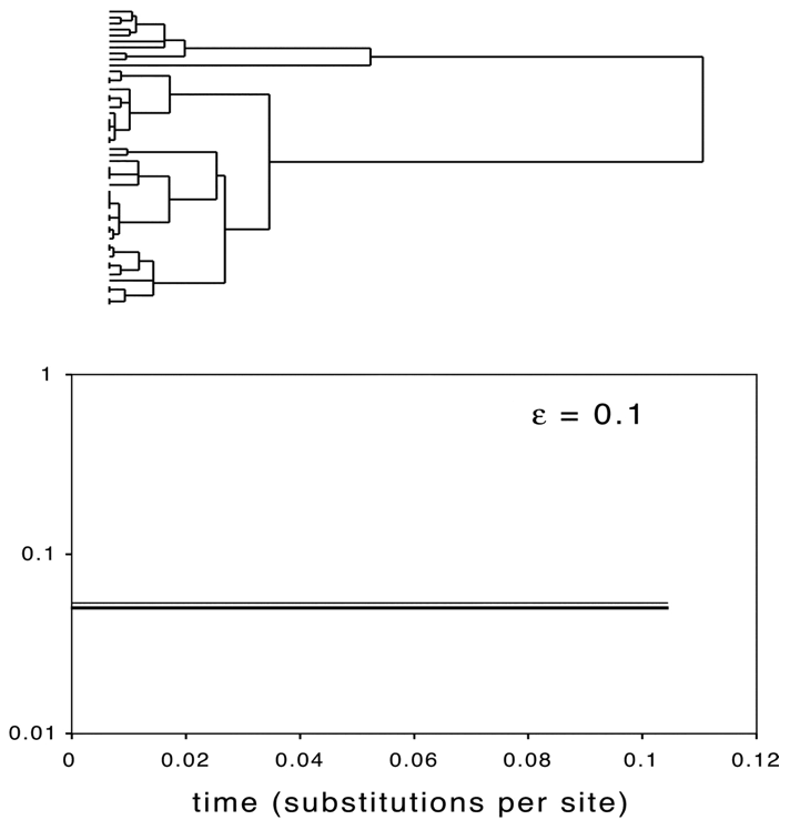
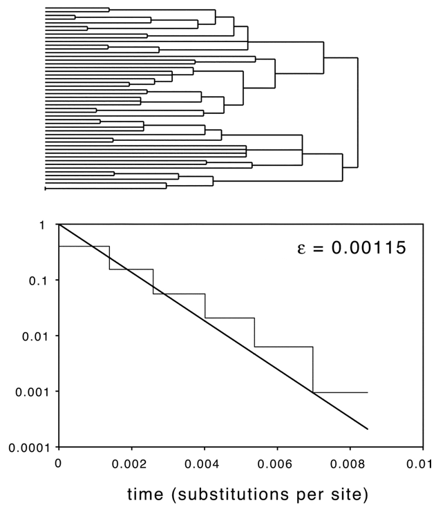
Adjacent intervals are grouped together to control the noise, which is the same thing the simulation above does with its time windows.

The Bayesian skyline plot

• The tree is not known either. It is estimated from the same sequences, and it is uncertain.
• The Bayesian skyline plot (Drummond et al., 2005) samples trees and population histories together with MCMC, so the shaded band shows genuine uncertainty in the history.
• The population history is allowed a fixed number of steps, and the analysis integrates over where the steps fall.

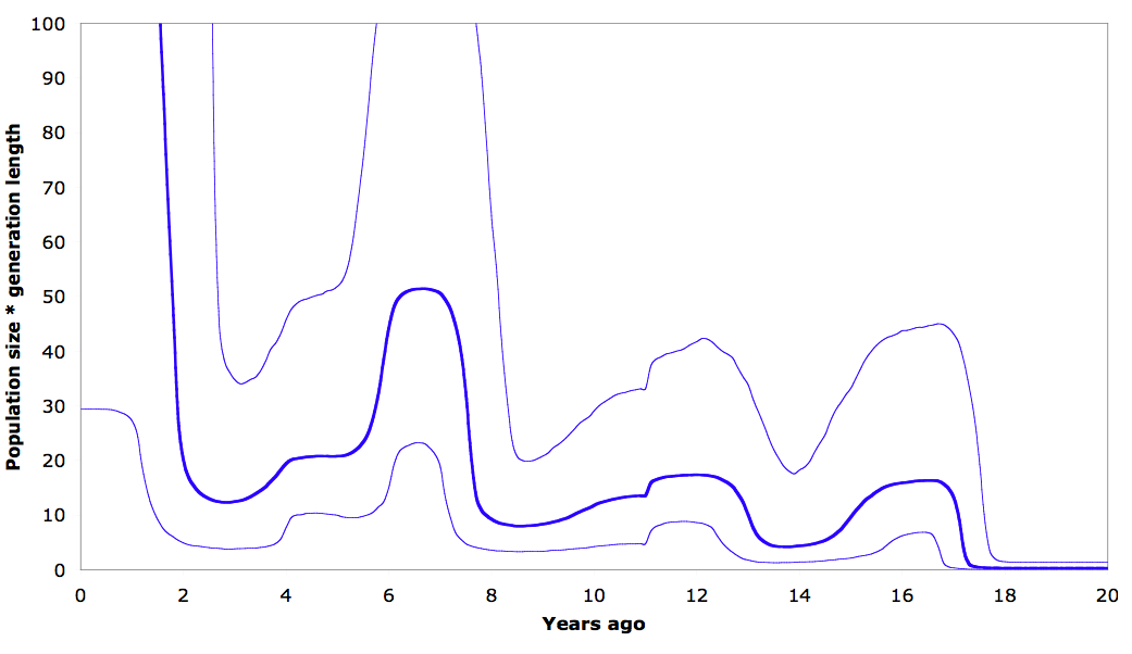
Human population history from mitochondrial DNA

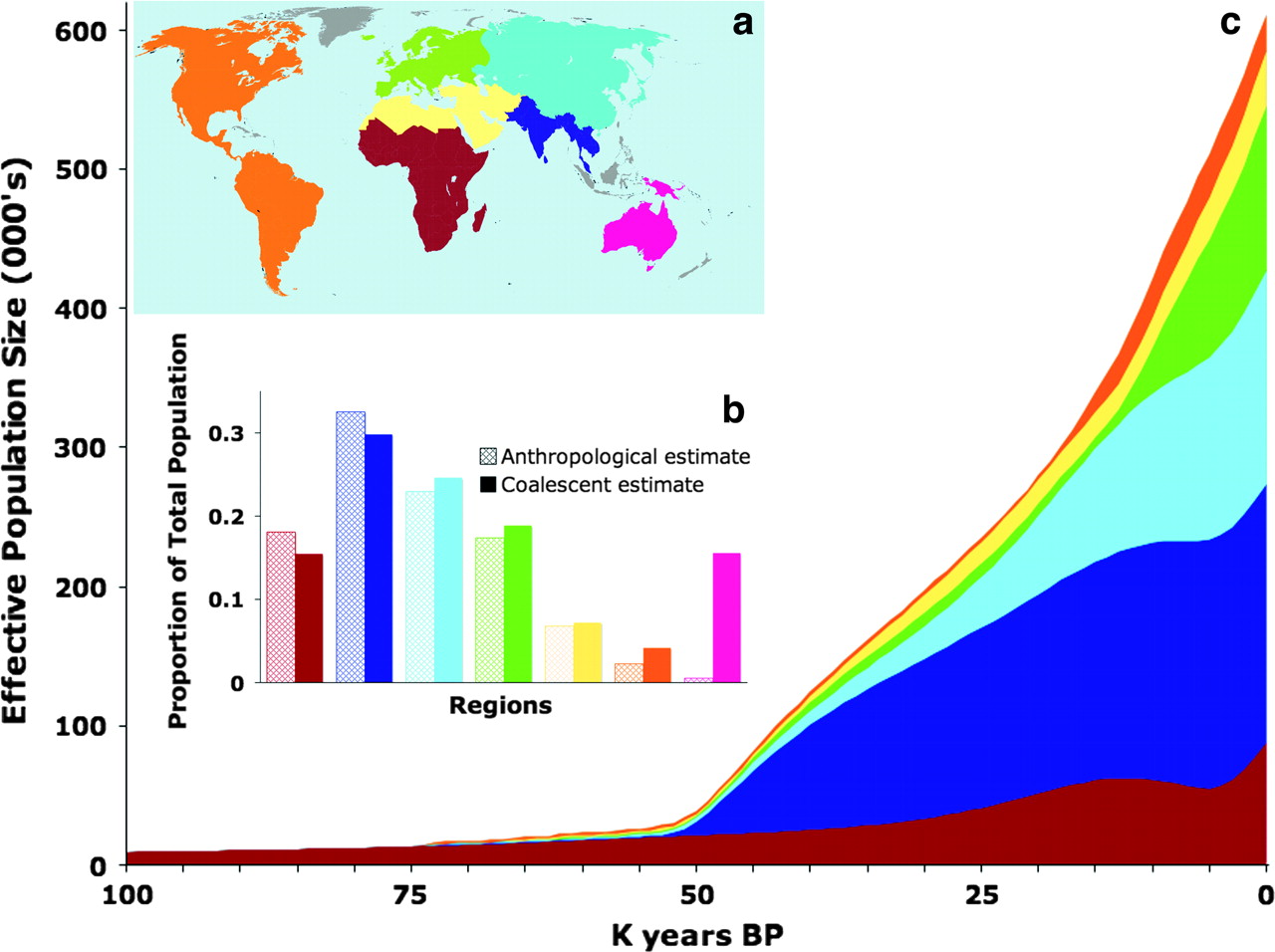
Mitochondrial sequences alone recover the expansion of human populations out of Africa, with the timing and the relative sizes of regional populations falling out of the tree shapes.

The origin of the HIV-1 pandemic

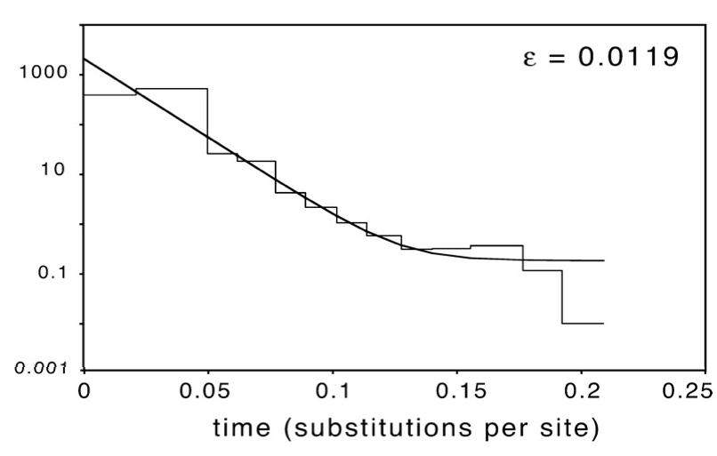
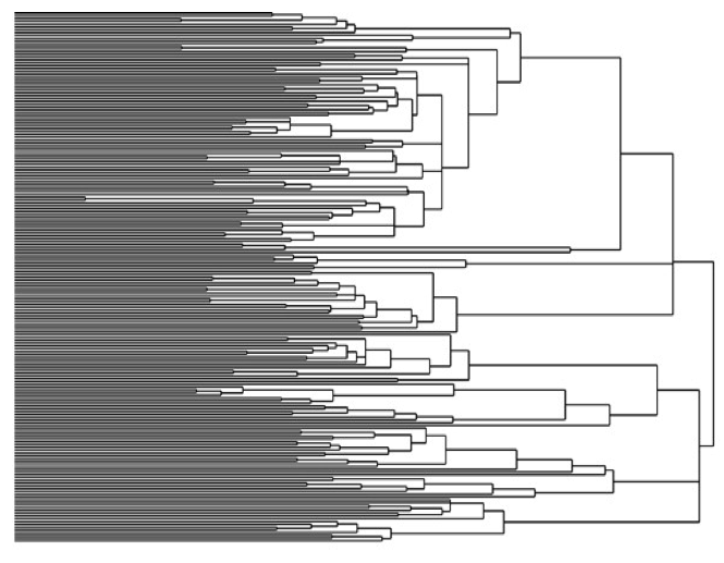
HIV-1 group M. The star-like tree on the right is the signature of a population that grew explosively, and the skyline plot on the left dates the start of that growth to the early twentieth century, decades before the disease was recognised.

Seasonal influenza

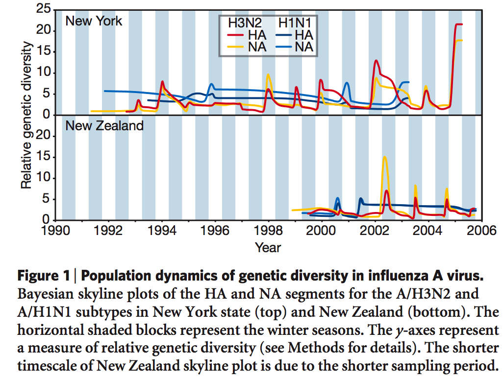
Genetic diversity in influenza A rises and falls every year. Each winter epidemic is a bottleneck, and the virus that seeds the next season descends from a small fraction of the previous one.

Does it agree with what we already know?

Dengue 4 in Puerto Rico. The blue band is estimated from virus genomes alone; the bars are reported cases:

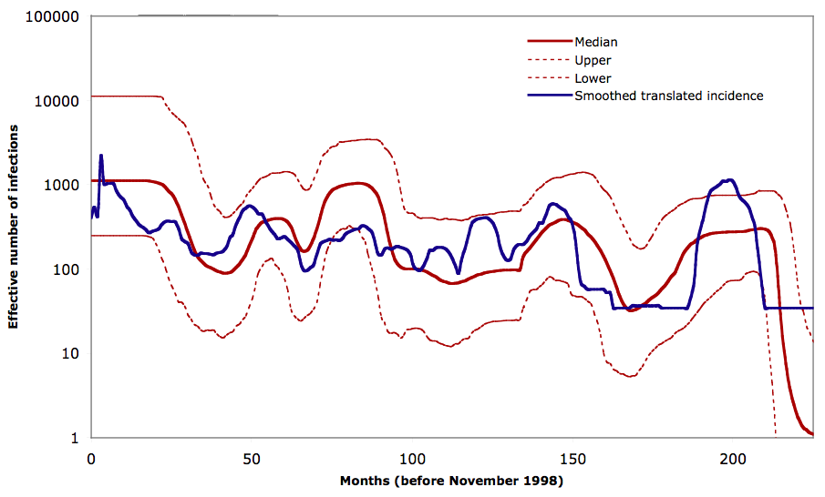
Genomes and surveillance data are independent sources, and they agree. That is the strongest kind of check available for a method whose answer concerns the unobserved past.

How much data does it take?

480 sequences, 1 locus

16 sequences from each of 32 loci

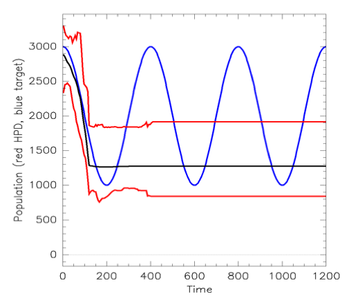
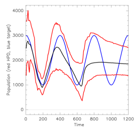
A single locus gives you one tree, and one tree is one realisation of a random process. Many independent loci give many trees, and only then does a bottleneck become clearly detectable.

What can go wrong

• Population structure looks like population decline. If a sample comes from several subpopulations that rarely exchange migrants, lineages cannot coalesce until they meet, which stretches the deep tree and mimics a large ancestral population.
• Selection breaks the assumptions. A selective sweep drags a whole region to a recent common ancestor, which looks exactly like a bottleneck.
• Sampling is rarely random. Sequences from an outbreak investigation are collected because they are related to each other.
• What is estimated is the effective population size. It is the size of an idealised Wright-Fisher population that would produce the observed variation, and it is usually much smaller than a census count.

Summary

• The coalescent traces a sample backwards in time. A pair of lineages meets at rate $1/N$ per generation, so waiting times are long in large populations and short in small ones.
• This makes the coalescent a tree prior: it assigns a probability to any genealogy, given a population history.
• Run the argument the other way and the shape of a tree becomes an estimate of population size through time. A long wait between branching events means the population was large then.
• A single tree is a single realisation of a random process, so the answer must be a distribution. The Bayesian skyline plot samples trees and histories together.
• This has recovered human expansion out of Africa, dated the origin of the HIV pandemic, and tracked seasonal influenza bottlenecks, from sequence data alone.
• The assumptions matter: neutrality, random sampling and a well-mixed population. Structure and selection can both counterfeit a demographic signal.

Recommended Reading

Also useful:

• Rosenberg & Nordborg (2002), "Genealogical trees, coalescent theory and the analysis of genetic polymorphisms", Nature Reviews Genetics 3:380–390.
• Ho & Shapiro (2011), "Skyline-plot methods for estimating demographic history from nucleotide sequences", Molecular Ecology Resources 11:423–434.