Before you can fit a model, you need a model
Last week in the lab, one line of R fit Brownian motion to finch beaks. This lecture is what that line assumes.
What this lecture is for
In the lab you ran lines like:
fitContinuous(tree, beakD, model = "BM")
Both rest on a single assumption: that the trait performs a random walk in continuous time along the branches of the tree. That random walk is Brownian motion (BM).
BM is the null model of trait evolution: the baseline that the contrast methods of last lecture assume, and the reference that every model next lecture is compared against.
One question to keep in mind:
When a trait "wanders" with no destination, what pattern does it leave at the tips of a tree, and how do we read the rate of wandering back out?
Three steps in this lecture
- BM as a process. A random walk, its rate $\sigma^2$, and why endpoints are normal.
- BM on a tree. Shared ancestry becomes the variance–covariance matrix $\mathbf{C}$; tips are multivariate normal.
- Estimating the rate. Contrasts, maximum likelihood, and REML recover $\sigma^2$ from the tips.
Step 2 is exactly the $\mathbf{C}$ you met in the comparative-methods lecture, now derived from first principles.
Brownian motion: the random walk
- The classic random walk: each instant the trait takes a small step in a random direction.
- Three rules define it:
- No bias toward any direction (steps average to zero).
- Each step is independent of every other step.
- Steps occur in continuous time, not discrete generations.
- Add up many small independent steps and, by the central limit theorem, the displacement is normally distributed.
Harmon (2019) PCM, Fig 3.1 (CC-BY-4.0).
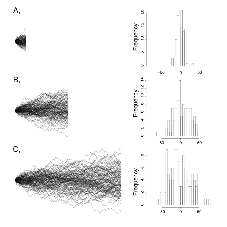
Try it yourself: watch the walk spread
Independent lineages from a common ancestor at value 0.
The grey band is the theoretical $\pm 2\sqrt{\sigma^2 t}$ envelope. The spread grows with $\sqrt{t}$; the mean stays put unless you add a trend $\mu$.
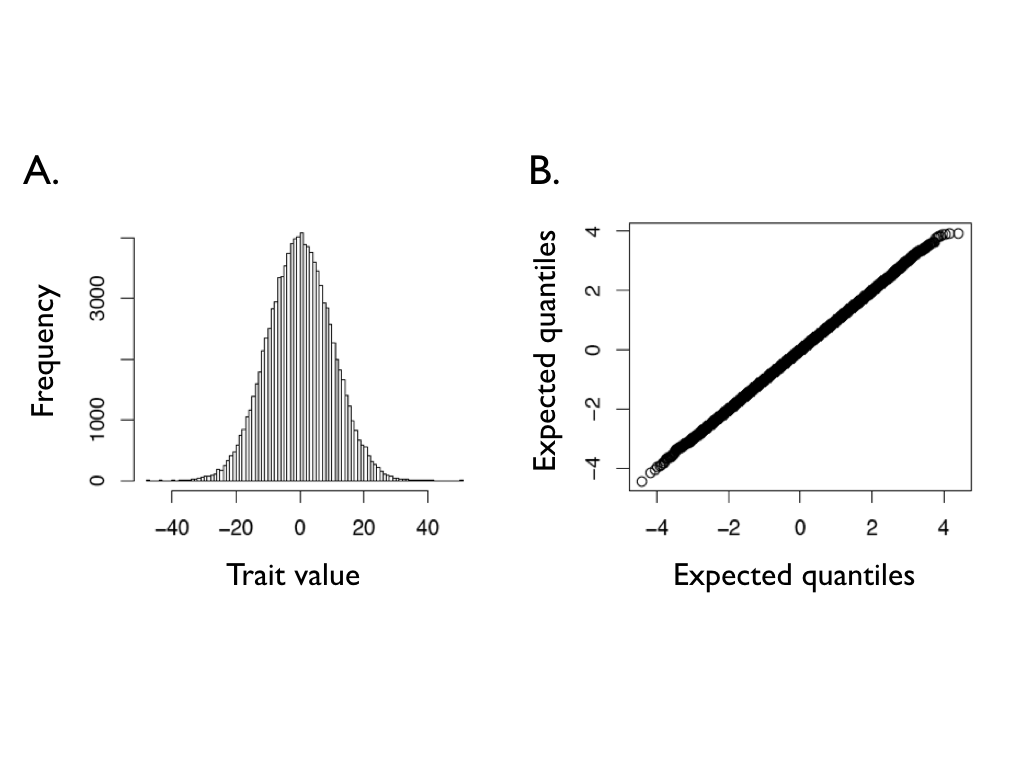
Many steps add up to a normal distribution
- Run the walk for time $t$ and record where each lineage ends up.
- The endpoints are normally distributed: $$X(t) \sim N\!\left(X(0),\; \sigma^2 t\right)$$
- The mean equals the starting value $X(0)$.
- The variance grows linearly with time: $\operatorname{Var}=\sigma^2 t$.
- This single result is the engine behind everything that follows.
Harmon (2019) PCM, Fig 3.2 (CC-BY-4.0).
The rate parameter $\sigma^2$
- $\sigma^2$ sets how much change accumulates per unit time. It is the one number BM has to estimate.
- After time $t$, the spread of trait values is $N(X(0),\,\sigma^2 t)$: higher $\sigma^2$ means a wider distribution.
- The mean stays at the starting value whatever the rate.
- Units matter: $\sigma^2$ is in (trait units)$^2$ per unit of branch length, so log-transforming a trait changes what $\sigma^2$ means.
Three defining properties of BM
The expected value never moves from $X(0)$. The walk has no destination.
$\operatorname{Var}=\sigma^2 t$. Long branches accumulate more change; the uncertainty fans out as $\sqrt{t}$.
Change in one interval is independent of, and normal like, change in any other. Non-overlapping branches evolve independently.
Property 3 is what makes independent contrasts work: differences between sister taxa are independent normal draws.
Why would a trait evolve by Brownian motion?
- BM is the mathematical twin of genetic drift. When change is neutral:
- a trait is influenced by many genes, each of small effect, and
- the trait does not affect fitness,
- But a BM-like pattern does not imply neutrality. Several selective regimes also produce BM at the macroevolutionary scale (next slide).
- This is why BM is a sensible null: it is what we expect from drift, and a useful baseline even when selection is at work.
Brownian motion can also arise under selection
- Three regimes produce a Brownian-like result across a phylogeny (each assumes selection is weak relative to drift over macroevolutionary time):
- 1. Fluctuating directional selection. The direction (and strength) of selection varies randomly from generation to generation, so over long spans it averages to a random walk.
- 2. Stabilizing selection toward a moving optimum. The optimum itself wanders randomly and the population tracks it.
- 3. Drift with weak selection. Selection is present but too weak relative to drift to leave a consistent directional trend.
- When selection is strong and persistent, it dominates drift and BM is no longer appropriate. That is the case for the Ornstein–Uhlenbeck model next lecture.
Brownian motion with a trend
- Add a directional drift parameter $\mu$ and the endpoints become: $$X(t) \sim N\!\left(X(0) + \mu t,\; \sigma^2 t\right)$$
- The mean now slides at rate $\mu$ while the spread still grows as $\sigma^2 t$ (try $\mu \ne 0$ in the simulator three slides back).
- The catch: on an ultrametric tree of living species only, all tips have the same age, so a trend in the mean and a shifted root value are confounded. The trend cannot be estimated from extant tips alone.
- Detecting a trend needs fossils (tips of different ages) or a strong trend relative to $\sigma^2$.
Brownian motion on a phylogeny
From a single walk to a tree of correlated walks
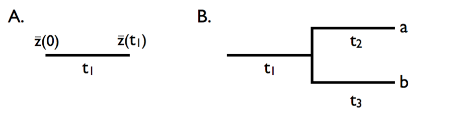
Evolving a trait down a tree
- On a single branch (A), the trait performs BM from the ancestral value $\bar{z}(0)$ to $\bar{z}(t_1)$.
- At a speciation event (B), the two daughter lineages start from the same ancestral value, then evolve independently.
- So two species share all the change that happened before they split, and nothing after.
- Shared history creates covariance; independent history after the split creates variance. This single idea builds the whole tip distribution.
Harmon (2019) PCM, Fig 3.4 (CC-BY-4.0).
Try it yourself: BM on a 8-tip tree (a traitgram)
Each lineage does its own BM down the branches. Sister lineages share their path until they split, then diverge.
Time runs left to right; the vertical axis is the trait value. Colour marks the two deep clades.
Notice how the two same-coloured tips in each "cherry" end up close together: shared ancestry makes related species resemble one another, even with no selection.
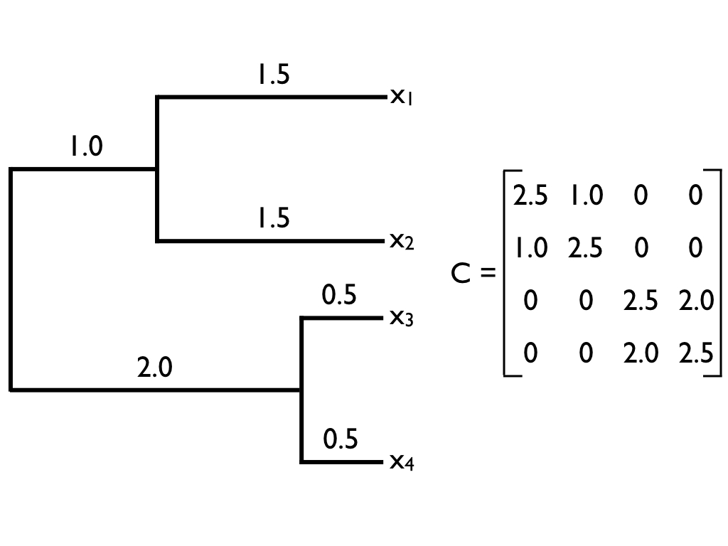
Shared ancestry becomes a covariance matrix $\mathbf{C}$
$\mathbf{C}_{ij}$ = shared branch length from the root to the common ancestor of $i$ and $j$
| A | B | C | D |
Diagonal = root-to-tip length (the variance of that tip). Off-diagonal = shared path (the covariance between two tips). A and B share the most; D shares nothing.
The tips are one big multivariate normal
- Stack the tip values into a vector $\mathbf{x}=(X_A,\dots,X_n)^\top$. Under BM they follow a multivariate normal: $$\mathbf{x} \sim \mathrm{MVN}\!\left(X(0)\,\mathbf{1},\; \sigma^2\,\mathbf{C}\right)$$
- Two parameters only: the root state $X(0)$ and the rate $\sigma^2$. The tree fixes $\mathbf{C}$.
- This is the likelihood. Everything else (contrasts, ML, REML, PGLS) is a different route to the same multivariate normal.
- For several traits at once, replace $\sigma^2$ with a rate matrix $\mathbf{R}$ (the multivariate BM of last lecture).
Harmon (2019) PCM, Fig 3.5 (CC-BY-4.0).
Winding back the clock: ancestral states
- Because the tips are multivariate normal, we can also estimate what the internal nodes most likely were.
- A node's estimate is an inverse-variance weighted average of its descendants: a short-branch descendant has drifted little, so it reflects the ancestor closely and counts more; a long-branch descendant counts less.
- Uncertainty grows toward the root: deeper nodes have wider intervals, and the root state is hardest to estimate.
- The same logic extends to multivariate traits, and to other models (OU, early burst) by swapping $\mathbf{C}$ for the model's own covariance.
Estimating the rate of evolution
Three routes to $\sigma^2$: contrasts, maximum likelihood, REML
Route 1: independent contrasts
- Recall from last lecture: a standardised contrast between sister taxa $i,j$ is $$c_{ij} = \frac{X_i - X_j}{\sqrt{v_i + v_j}} \sim N(0,\,\sigma^2)$$
- The contrasts are independent draws from $N(0,\sigma^2)$, so the rate is just their (mean) squared size: $$\hat{\sigma}^2_{\text{PIC}} = \frac{1}{n-1}\sum_k c_k^2$$
- Simple, fast, and exact under BM. This is what ape::pic() computes for you, and what you regressed in the lab.
- One subtlety: dividing by $n-1$ (not $n$) is the REML correction, accounting for having estimated the root state. More on that shortly.
Route 2: maximum likelihood
- Write down the multivariate-normal likelihood and find the $(\sigma^2, X(0))$ that maximise it.
- The likelihood surface (right) has a single peak: the maximum-likelihood estimate.
- This is what geiger::fitContinuous(model="BM") reports: sigsq ($\hat{\sigma}^2$) and z0 ($\hat{X}(0)$), plus the log-likelihood and AIC.
- The log-likelihood and parameter count are exactly what feed the AIC model comparison you will do next lecture.
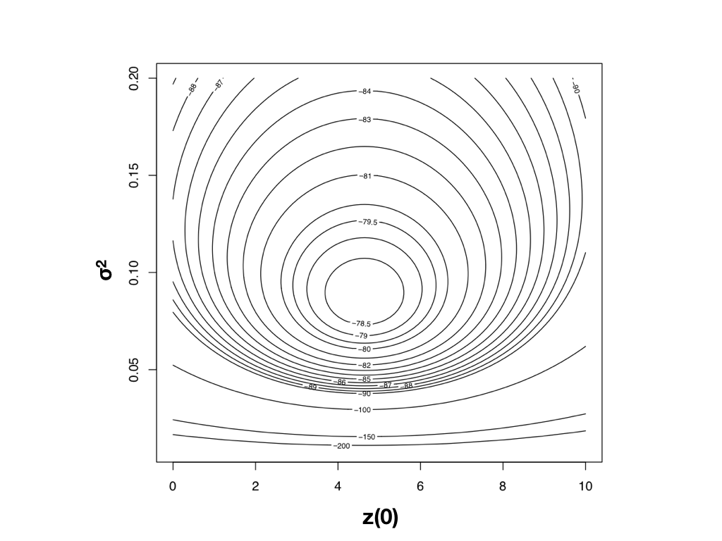
Harmon (2019) PCM, Fig 4.3 (CC-BY-4.0).
Try it yourself: where is the likelihood peak?
Data simulated under a true rate, then we plot the log-likelihood as a function of the candidate rate $\sigma^2$.
The MLE (red) is the rate that makes the observed contrasts most probable. With few contrasts it scatters widely around the truth; with many it homes in.
Hill-climbing to the maximum
- For most models there is no formula for the peak, so software takes iterative steps uphill.
- On a smooth, single-peaked surface (right), it converges in a handful of steps.
- Risk: getting trapped on a local optimum when the surface is rugged (common for OU and multi-rate models next lecture).
- Mitigations:
- multiple random starting points,
- simulated annealing,
- Bayesian MCMC, which explores the whole landscape rather than climbing one hill.
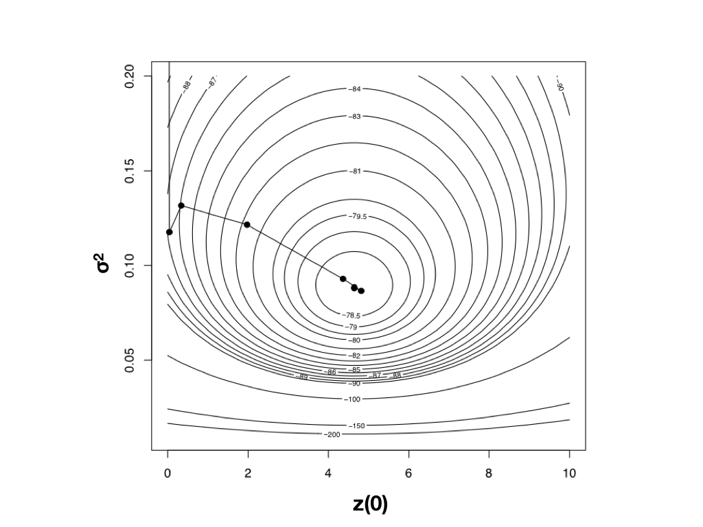
Harmon (2019) PCM, Fig 4.4 (CC-BY-4.0).
Route 3: restricted maximum likelihood (REML)
- Ordinary ML estimates the rate and the root state together, and the rate estimate comes out slightly biased (too small), because it does not pay for having estimated the root.
- REML maximises the likelihood of the contrasts instead of the raw data:
- it sidesteps the nuisance root-state parameter, and
- it gives a less biased estimate of the variance parameter $\sigma^2$.
- The contrast estimator $\hat{\sigma}^2_{\text{PIC}}=\frac{1}{n-1}\sum c_k^2$ is the REML estimate. Routes 1 and 3 are the same thing.
- REML is also cheaper: contrasts avoid inverting the full $n\times n$ matrix $\mathbf{C}$, which matters for large trees.
A worked fit: what fitContinuous returns
Fitting BM to a single continuous trait (here, log body size on a lizard phylogeny) returns four numbers that summarise the whole fit:
| output | meaning |
|---|---|
| sigsq | $\hat{\sigma}^2$, the rate of evolution |
| z0 | $\hat{X}(0)$, the estimated root state |
| lnL | maximised log-likelihood |
| AIC / AICc | fit penalised by parameter count, for model comparison |
Two free parameters here ($\sigma^2$ and $X(0)$), so $\mathrm{AIC}=2\cdot 2 - 2\ln L$.
Is Brownian motion a reasonable model?
- BM is a strong set of assumptions: no trend, a constant rate everywhere on the tree, and independent increments.
- Reasons it may fail:
- stabilizing selection holds a trait near an optimum (variance stops growing): use OU;
- a rate that slows after a radiation: use early burst;
- some clades evolve faster than others: use a multi-rate model;
- phylogenetic signal weaker than BM predicts: estimate Pagel's $\lambda$.
- How to decide: fit the alternatives and compare with AIC or Bayes factors. Never accept BM just because it ran.
- That comparison is exactly the workflow you used in the lab, and the subject of the next lecture.
Discussion
- If the PIC estimator $\frac{1}{n-1}\sum c_k^2$ gives the rate directly, why bother with maximum likelihood or Bayesian approaches at all?
- What are the arguments for log-transforming sizes, masses, and lengths before a comparative analysis?
- On a tree of only living species, a slow evolutionary trend cannot be distinguished from noise. Why, and what kind of data would break the tie?
- Ancestral states under BM are pulled toward the mean of the tips. When would that make a reconstructed root state misleading?
- How would you decide whether Brownian motion is a reasonable model for a given trait?
Recommended Reading
- Chapter 8: Traits and Comparative Methods
- Chapter 3: Introduction to Brownian Motion
- Chapter 4: Fitting Brownian Motion Models to Single Characters