When does evolution leave Brownian motion behind?
In the lab, fitContinuous compared BM, OU, EB and $\lambda$ by AIC. Why four models, and what does each one actually mean?
What this lecture is for
Brownian motion is the null. It says a trait wanders with no destination, at one constant rate, everywhere on the tree. Real traits often do something more interesting:
- Constraint. A trait is held near an optimum and stops wandering: the Ornstein–Uhlenbeck model.
- Bursts. A trait diversifies fast early then slows: the early-burst model.
- Lost signal. Relatives resemble each other less than the tree predicts: Pagel's transformations.
Each is BM plus one extra parameter. Setting that parameter to its default value recovers BM exactly, so each is a testable departure from the null.
Three families of model
- Reshape the tree. Pagel's $\lambda$, $\delta$, $\kappa$; multi-rate models.
- Change the process. Ornstein–Uhlenbeck; early burst.
- Discrete traits. The Mk model and stochastic mapping.
Choosing between them is a model-selection problem: fit each, then compare with AIC, exactly the aicw() step from the lab.
Every model here is compared against the null
- Each model returns a log-likelihood and a parameter count $k$. From these, recall (lecture 11): $$\mathrm{AIC} = 2k - 2\ln L, \qquad \mathrm{AIC_c} = \mathrm{AIC} + \frac{2k(k+1)}{n-k-1}$$
- Because BM is nested inside most of these models (set $\alpha=0$, $r=0$, or $\lambda=1$), we can also use a likelihood-ratio test.
- AIC turns the fits into weights: the relative probability that each model is the best in the set. That is what geiger::aicw() reports.
- Keep this frame in mind: the rest of the lecture is a menu of alternatives, and the last ingredient is always "compared to what?"
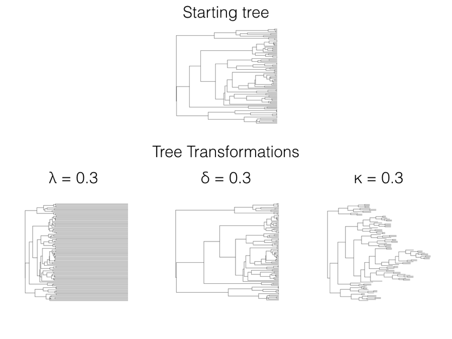
Reshaping the tree: Pagel's transformations
Three transformations of $\mathbf{C}$
- Pagel proposed three ways to stretch and squeeze the variance–covariance matrix $\mathbf{C}$ before fitting BM.
- Each has one parameter that, set to 1, recovers the original BM tree:
- $\lambda$ (lambda): phylogenetic signal,
- $\delta$ (delta): the tempo of evolution through time,
- $\kappa$ (kappa): gradual versus speciational change.
- Fitting the parameter and comparing to $1$ tests whether the trait obeys BM on the true tree.
Harmon (2019) PCM, Fig 6.1 (CC-BY-4.0).
Try it yourself: Pagel's $\lambda$ and phylogenetic signal
$\lambda$ multiplies the internal (shared) branches, leaving the tips at the present.
$\lambda$ was one of the four models you fit in the lab. A fitted $\lambda<1$ says the trait carries less phylogenetic signal than Brownian motion on this tree would produce.
Phylogenetic signal, in one number
- Phylogenetic signal is the tendency for related species to resemble one another. Pagel's $\lambda$ is one way to quantify it.
- Interpreting a fitted $\lambda$:
- $\lambda \approx 1$: relatives are as similar as BM on the tree predicts.
- $\lambda \approx 0$: the trait is effectively independent of the phylogeny.
- $\lambda > 1$ is occasionally seen and usually signals model misfit.
- Blomberg's $K$ is a related statistic: $K>1$ means relatives are more similar than BM predicts (conserved); $K<1$ means less.
- Low signal is itself informative: it suggests strong selection, measurement error, or a trait responding fast to the current environment, the very situation where ignoring phylogeny is least harmful (recall Felsenstein's caveat).
Pagel's $\delta$ and $\kappa$
Raises node heights to the power $\delta$, rescaling when change happens.
- $\delta=1$: unchanged BM.
- $\delta<1$: change concentrated early (deep branches do more work).
- $\delta>1$: change concentrated late (recent branches do more).
Raises each branch length to the power $\kappa$.
- $\kappa=1$: standard BM (change $\propto$ time).
- $\kappa=0$: all branches length 1; change depends only on the number of speciation events, not on time (punctuated evolution).
Compare the $\delta=0.3$ and $\kappa=0.3$ panels in the figure two slides back: $\delta$ moves the splits in time, while $\kappa$ pushes the model toward "change happens at speciation."
Try it yourself: Pagel's $\kappa$
$\kappa$ raises each branch length to the power $\kappa$. The horizontal axis is now expected change, not time.
As $\kappa\to0$ the long deep branches shrink toward the short ones, and tips reached through more speciation events end up further along the change axis: a model of punctuated evolution.
Different rates in different clades
- BM assumes a single rate $\sigma^2$ across the whole tree. What if one clade evolves faster?
- Three ways to test:
- Contrast-based rate test: compare the spread of squared contrasts between clades.
- ML + AIC: fit a model with a separate $\sigma^2$ per clade and compare to single-rate BM.
- Bayesian MCMC: let every branch have its own rate; the posterior flags rate shifts.
- Caveat: methods 1 and 2 need the clades to be specified in advance. Scanning every clade and keeping the most significant inflates false positives.
Harmon (2019) PCM, Fig 6.2 (CC-BY-4.0).
Constraint: the Ornstein–Uhlenbeck model
A rubber band toward an optimum
- The Ornstein–Uhlenbeck (OU) model is BM plus a pull toward an optimum $\theta$: $$dX = \underbrace{\alpha(\theta - X)\,dt}_{\text{pull to optimum}} + \underbrace{\sigma\,dW}_{\text{random walk}}$$
- $\alpha$ is the strength of the pull. The further $X$ strays from $\theta$, the harder it is pulled back.
- This is the model of stabilizing selection: a trait kept near an adaptive peak (right).
- Special case: $\alpha=0$ removes the pull and OU collapses to plain BM. So OU nests BM.
Harmon (2019) PCM, Fig 6.3 (CC-BY-4.0).
Try it yourself: the OU pull
Lineages start away from the optimum $\theta$ (green line) and are pulled toward it as they wander.
Set $\alpha=0$ for pure BM (the spread keeps growing). Increase $\alpha$ and the variance reaches a ceiling $\sigma^2/2\alpha$: the past is forgotten.
Properties of the OU model
Unlike BM, the variance does not grow forever; it approaches an equilibrium $\sigma^2/2\alpha$. Once divergence exceeds a few phylogenetic half-lives the trait reaches this equilibrium and further time adds little difference; on short branches OU still behaves like BM.
The phylogenetic half-life $\ln 2/\alpha$ says how fast ancestry is forgotten. Large $\alpha$ means the tree barely matters.
OU is easy to over-fit on small trees, and measurement error mimics a high $\alpha$. A favourable AIC is not proof of an optimum.
OU was the model most often favoured in the lab's finch-beak comparison: beak dimensions behave as if held near an adaptive optimum.
Multi-peak OU: many optima on one tree
- Let different parts of the tree be pulled toward different optima $\theta_1,\theta_2,\dots$ This is the Hansen model.
- Paint the branches with regimes; each regime has its own peak in trait space. Lineages sharing a regime are drawn to the same point.
- This formalises Simpson's "adaptive zones": shifts between peaks are shifts between adaptive strategies.
- When independent lineages are pulled to the same peak, the model captures convergence, exactly the test behind the Caribbean Anolis result from last lecture (Mahler et al. 2013).
Bursts: adaptive radiation
The early-burst model
- An opportunity opens (a new island, a key innovation, a mass extinction). Lineages diversify fast to fill empty niches, then slow as niches fill.
- The rate decays through time: $$\sigma^2(t) = \sigma^2_0\, e^{rt}, \quad r<0$$
- Most disparity accumulates early; the tips are relatively similar.
$r=0$ is constant-rate BM. As $r$ becomes more negative, the rate collapses early and the accumulated disparity flattens off: the signature of an early burst.
Peak shifts and punctuated change
- Punctuated models picture long stasis broken by brief bursts of change, often at speciation or at a shift in selective regime.
- The bursts can be modelled as occurring:
- at random points,
- at fixed intervals, or
- linked to changes in another trait on the tree.
- Like the multi-rate methods, these identify parts of the tree evolving differently from the rest.
- Linking a peak shift in one trait to changes in another is powerful but risky: with enough traits, some apparent association is almost guaranteed by chance.
Choosing among the models
The lab's fitContinuous + aicw step, formalised
Try it yourself: AIC weights
Four models fit to one trait. Set each log-likelihood; weights update live.
$w_i = \dfrac{e^{-\Delta_i/2}}{\sum_j e^{-\Delta_j/2}}$ where $\Delta_i = \mathrm{AIC}_i - \mathrm{AIC}_{\min}$. A higher likelihood helps, but the extra parameter in OU/EB/$\lambda$ must improve the fit enough to offset its AIC penalty.
What does this look like on real data?
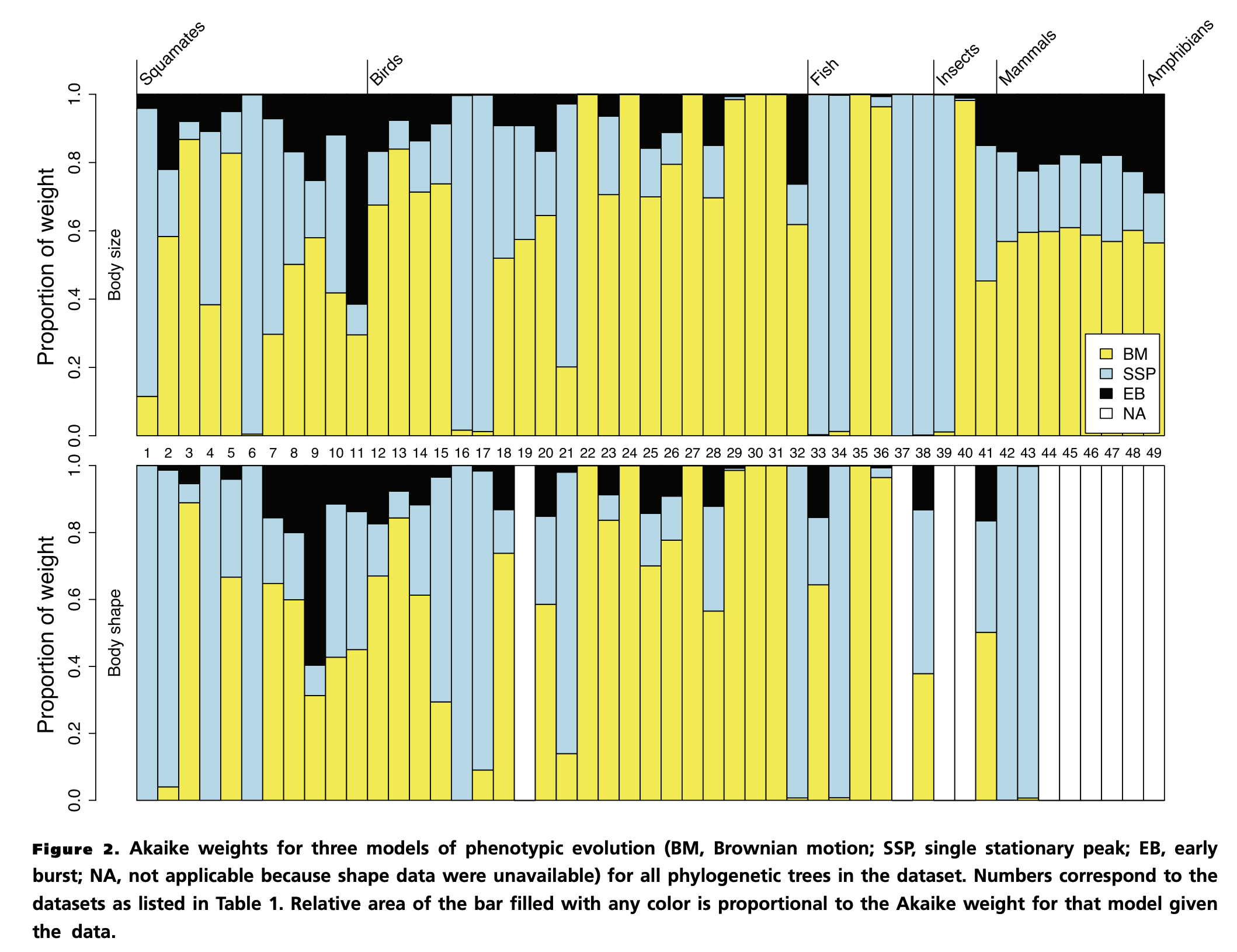
Harmon et al. (2010) Evolution 64: 2385–2396, Fig 2.
- Early burst (black) is almost absent: best-supported in only ~2 of 49 datasets, despite Simpson's adaptive-radiation prediction.
- Body size is dominated by OU (blue); body shape by BM (yellow). Bounded vs diffusive signatures.
- The same Akaike-weight calculation you just played with, run across the empirical literature.
Model selection: cautions
- The best model in a set is not necessarily a good model. AIC ranks the candidates you supplied; it cannot point to a model you did not fit.
- OU and early burst are easily over-fit on small trees, and measurement error can masquerade as OU. Treat a modest AIC advantage with scepticism.
- Check model adequacy, not just relative fit: simulate data under the winning model and ask whether it reproduces features of the real data.
- Report the weights, not just the winner. Two models within a couple of AIC units are effectively tied; choosing one and ignoring the other overstates certainty.
Discrete characters
When the trait is a category, not a number
- Many traits are discrete: present/absent, 2/3/4 colour morphs, diet category, limbed/limbless.
- These have no meaningful average, so BM and contrasts do not apply.
- Instead, model evolution as jumps between states along the branches, using a continuous-time Markov chain.
- This is the same modelling approach used for DNA substitution earlier in the course, now applied to phenotypes.
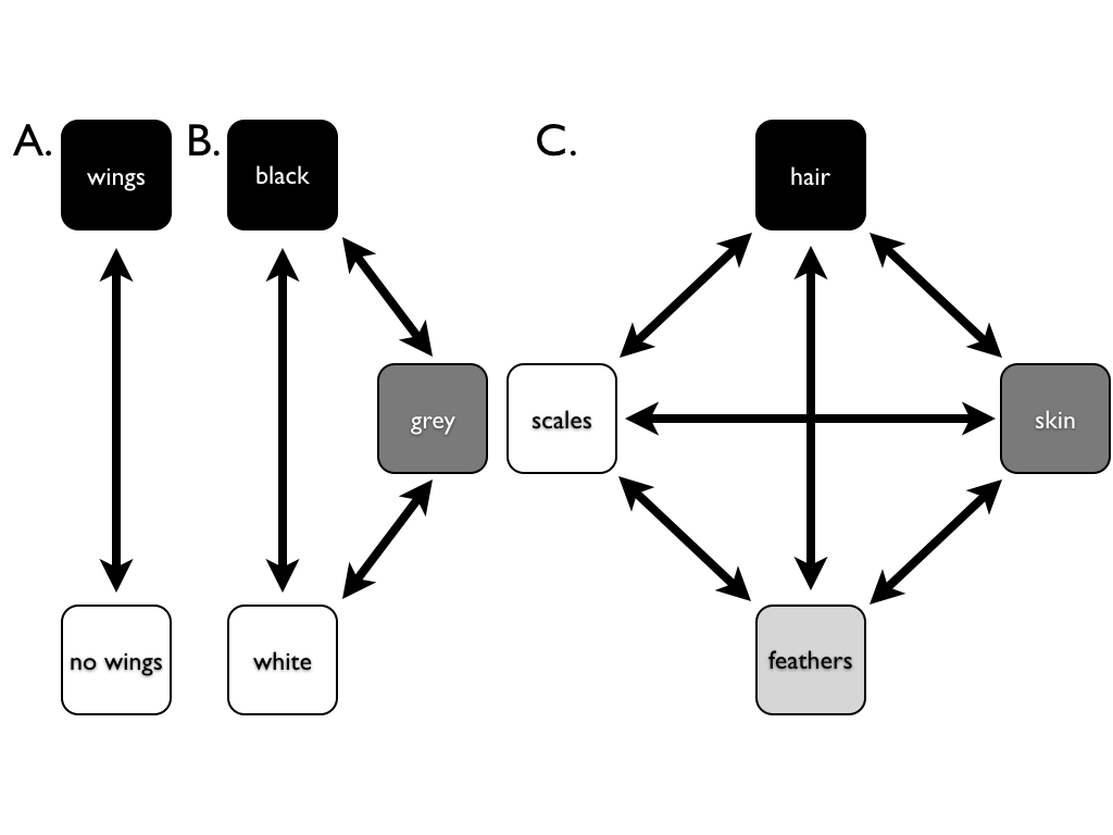
Harmon (2019) PCM, Fig 7.3 (CC-BY-4.0).
The Mk model
- The Mk model (Lewis 2001) describes a character with $k$ states changing at constant rates, a direct generalisation of the Jukes–Cantor model for DNA.
- Rates live in a transition matrix $\mathbf{Q}$. For $k=2$: $$\mathbf{Q} = \begin{pmatrix} -q_{01} & q_{01} \\ q_{10} & -q_{10} \end{pmatrix}$$
- The two flavours you fit in the lab:
- ER (equal rates): $q_{01}=q_{10}$, one rate.
- ARD (all rates different): each transition its own rate.
- More states or asymmetric rates simply add parameters to $\mathbf{Q}$; compare them with AIC, as before.
Harmon (2019) PCM, Fig 7.4 (CC-BY-4.0).
Try it yourself: simulate Mk on a tree
A binary trait (state 0 / state 1) evolves down the branches. Each branch is coloured by its current state.
Raise $q$ and transitions pile up; the same state can be reached independently on different branches (homoplasy). With ARD, state 1 tends to revert to state 0.
Computing the likelihood: pruning
- A single simulation is easy; the likelihood sums over all possible histories, which is astronomically many.
- Felsenstein's pruning algorithm makes it tractable: work from the tips to the root, storing at each node the probability of the data below it, for each possible state.
- At each node, combine the two daughter probabilities using $\mathbf{Q}$ and the branch lengths; recurse down to the root.
- This is the same algorithm used for DNA substitution models earlier in the course; only the states and $\mathbf{Q}$ differ.
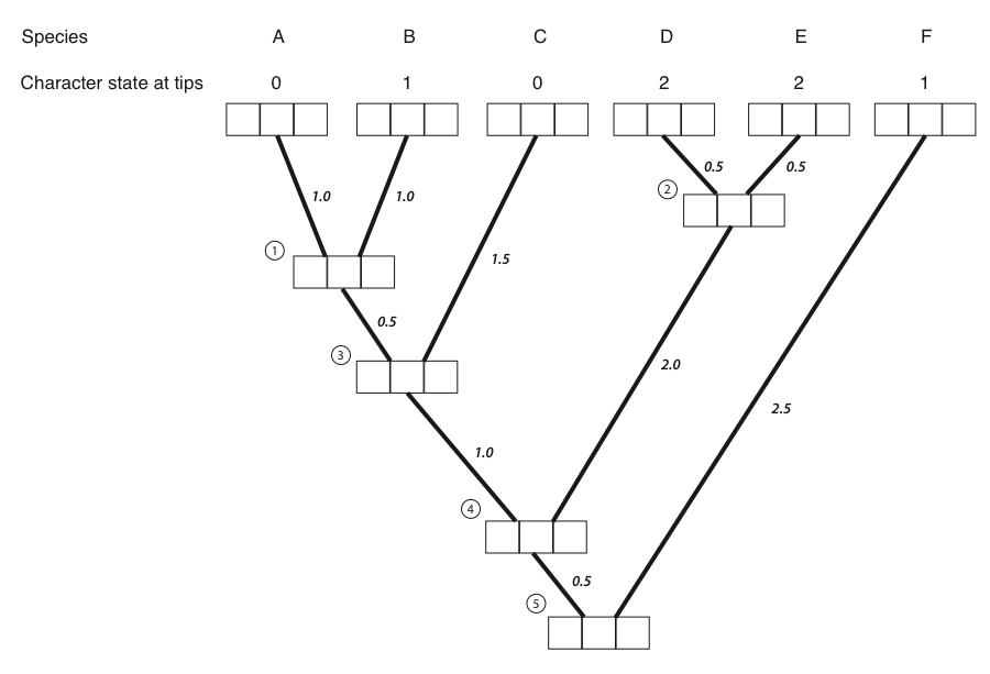
Harmon (2019) PCM, Fig 8.4 (CC-BY-4.0).
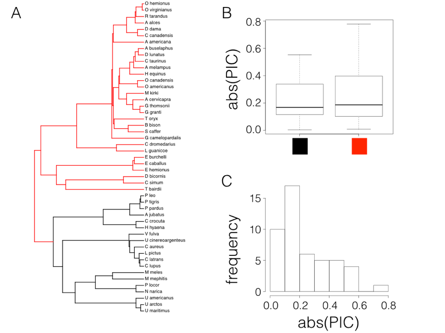
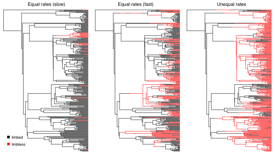
A real example: the evolution of limblessness
- Squamate reptiles (lizards and snakes) have lost their limbs many times independently: snakes, but also numerous lizard lineages.
- Fitting an Mk model and reconstructing ancestral states shows limblessness (red) scattered across the tree, not confined to one clade.
- Each red patch on a black background is an independent transition: a striking case of convergent evolution in a discrete trait.
- The same fit also estimates whether the limbed→limbless transition is effectively irreversible: regaining limbs is rare or impossible.
Harmon (2019) PCM, Fig 8.2 (CC-BY-4.0).
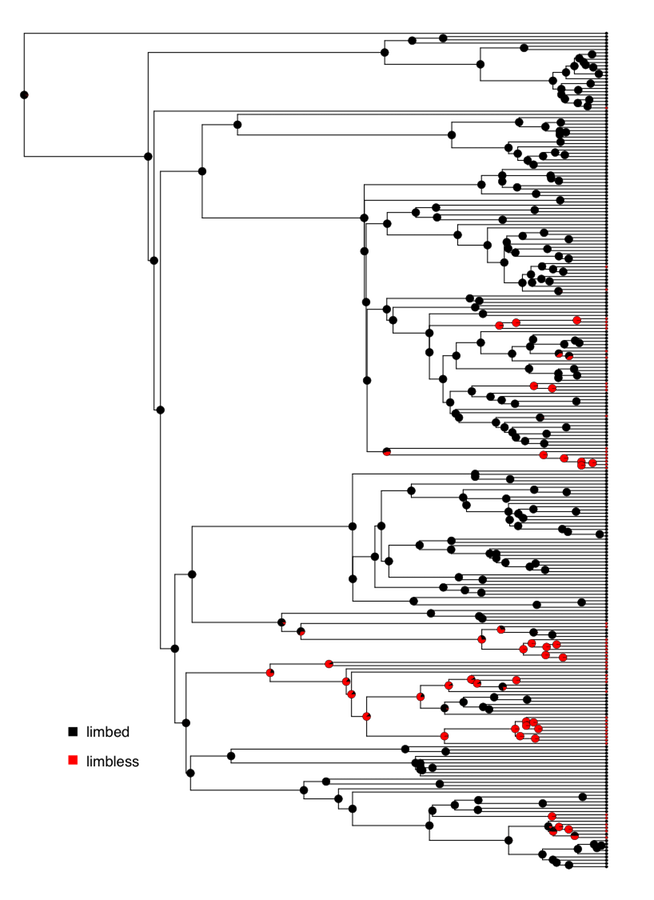
Stochastic character mapping
- Point estimates of ancestral states hide their uncertainty. Stochastic character mapping (SIMMAP) samples entire histories consistent with the tips and the fitted $\mathbf{Q}$.
- In the lab you ran make.simmap(..., nsim = 100): 100 sampled histories, each a complete painting of states along every branch.
- Summarising the 100 maps gives, at every node, the posterior probability of each state, shown as pie charts on the tree.
- Why it matters: a single reconstruction can look confident even when the data barely constrain a node. The spread across sampled maps is the honest measure of what we know.
- The same idea underlies counting how many times a trait was gained or lost: average those counts over the sampled histories rather than trusting one reconstruction.
State-dependent diversification (SSE)
- Does a trait change the rate of speciation or extinction? SSE models join an Mk model to a birth–death model so the diversification rate can depend on the state.
- An alphabet of variants:
- BiSSE: binary-state speciation and extinction,
- HiSSE: adds a hidden state to absorb unmeasured rate variation,
- MuSSE: multiple states.
- Use when the question is explicitly "does having this trait make a lineage diversify faster?"
- Caution: SSE models are prone to false positives. Any clade that happens to be both species-rich and trait-biased can trigger a spurious signal. HiSSE and careful null models exist precisely because of this.
Summary: a menu of models beyond BM
| Model | What it captures | Key parameter(s) | Recovers BM when |
|---|---|---|---|
| Pagel's $\lambda$ | Phylogenetic signal | $\lambda \in [0,1]$ | $\lambda=1$ |
| Pagel's $\delta$ | Tempo through time | $\delta$ (node-height power) | $\delta=1$ |
| Pagel's $\kappa$ | Gradual vs speciational | $\kappa$ (branch-length power) | $\kappa=1$ |
| Multi-rate BM | Rate varies across clades | $\sigma^2_1,\sigma^2_2,\dots$ | all rates equal |
| OU | Stabilizing selection | $\alpha$ (pull), $\theta$ (optimum) | $\alpha=0$ |
| Early burst | Adaptive radiation | $r$ (rate decay) | $r=0$ |
| Mk | Discrete-character evolution | transition rate(s) in $\mathbf{Q}$ | (continuous analogue) |
| SSE (BiSSE, HiSSE...) | Trait-dependent diversification | state-specific $\lambda,\mu$ | (birth–death analogue) |
Each continuous model is BM plus one parameter. Fit them, read off log-likelihoods, and let AIC weights decide, exactly the lab workflow.
Discussion
- If you do not know in advance which clade evolves at a different rate, what are the risks of testing every clade and keeping the most significant?
- A fitted OU model beats BM by a few AIC units on a tree of 20 species. What would you check before believing the trait is under stabilizing selection?
- For what reasons might Pagel's $\lambda$, $\delta$ and $\kappa$ be less popular today than process-based models like OU?
- Under the early-burst model, why do we expect the rate to slow over time, and what would the tips look like if it did?
- Stochastic mapping returns 100 different histories for the same data. Why is that spread more useful than a single "best" reconstruction?
Recommended Reading
- Chapter 8: Traits and Comparative Methods
- Chapter 6: Beyond Brownian Motion (OU, early burst)
- Chapter 7: Introduction to Discrete Characters
- Chapter 8: Fitting Models of Discrete Character Evolution