Where we are going
- A phylogeny is something we estimate, not something we observe. Any estimate comes with uncertainty, and we would like to measure it.
- Part 1. Probability as a measure of belief, and Bayes' theorem.
- Part 2. What a Bayesian phylogenetic analysis is actually asking.
- Part 3. How a computer answers the question: Markov chain Monte Carlo (MCMC).
- Part 4. Reading the output, and what a posterior probability on a branch means.
Later lectures add the time axis (molecular clocks, L9) and then fill in the biology of the tree priors: the coalescent (L10), the multispecies coalescent (L11) and birth-death models (L12).
Part 1: Reasoning under uncertainty
Suppose some dark night a policeman walks down a street. He hears a burglar alarm, looks across the street, and sees a jewelry store with a broken window. Then a gentleman wearing a mask comes crawling out of the window, carrying a bag full of jewelry. The policeman decides immediately that the gentleman is a thief. How does he decide this?E. T. Jaynes, Probability Theory: The Logic of Science
Strict logic is not enough
Deductive logic only licenses conclusions of this form:
if $A$ is true, then $B$ is true
$A$ is true
$B$ is true
The policeman has no such certainty. What he actually uses is:
if $A$ is true, then $B$ is likely
$B$ is true
$A$ is likely
This is exactly the situation of a biologist with an alignment and a question about ancestry.
Probability as degree of belief
$P(A \mid B)$ is how strongly we should believe $A$, given that we know $B$. It is a measure of the state of our knowledge, not a property of the world.
- $P = 0$ means certainly false, $P = 1$ means certainly true, and everything in between is a degree of confidence.
- The same statement can have different probabilities for different people, if they know different things.
- This is what lets us say "the probability that humans and chimpanzees are each other's closest relatives is 0.93". There is no repeatable experiment there, only one history and our uncertainty about it. We will compute exactly that number in Part 3.
Bayes' theorem
One equation connects what we believed before the data to what we should believe after:
$$\color{cyan}{P(H \mid D)} = \frac{\color{orange}{P(D \mid H)}\;\color{#ff9c9c}{P(H)}}{\color{lime}{P(D)}}$$
- Posterior, $P(H \mid D)$
- How plausible the hypothesis $H$ is once we have seen the data. This is the answer we want.
- Likelihood, $P(D \mid H)$
- If $H$ were true, how probable would these data be? This is where the evolutionary model enters.
- Prior, $P(H)$
- How plausible $H$ was before we looked at the data.
- Marginal likelihood, $P(D)$
- A normalising constant. It does not depend on $H$, and Part 3 shows we never need to compute it.
The same idea in words
posterior $\;\propto\;$ likelihood $\times$ prior
- Hypotheses that explain the data well are promoted.
- Hypotheses that were implausible to begin with are demoted.
- The posterior is the compromise, and it is a full distribution, not a single answer. That distribution is the measure of uncertainty.
Try it yourself: updating a belief
You want the frequency of an allele in a population. You have some prior expectation, and you genotype $n$ individuals, of which $k$ carry the allele.
With little data the prior dominates. With plenty of data the likelihood dominates and the choice of prior stops mattering.
A word about priors
- A prior is not an optional extra. Inference without assumptions is not possible, and the prior is where the assumptions are written down explicitly.
- Priors are how existing knowledge enters an analysis: fossil ages, known mutation rates, plausible population sizes.
- A prior that is too confident will not be overturned by weak data. This is a feature when the prior is well founded, and a problem when it is not.
- In phylogenetics the most consequential prior is the tree prior, which we come to next.
Always report your priors, and always check whether they matter.
Part 2: The Bayesian phylogenetics question
What are the unknowns?
The data are an alignment. Essentially everything else is unknown:
- The tree, $\color{red}{g}$
- Its topology, who is related to whom, a discrete unknown with an enormous number of possible values; and its branch lengths, how much evolution or how much time separates the lineages.
- Substitution model parameters, $\color{#b8860b}{Q}$
- Relative rates of the different nucleotide changes, rate variation among sites.
- Tree prior parameters, $\color{blue}{\Theta}$
- Population sizes, speciation and extinction rates, migration rates.

We want a posterior distribution over all of it at once.
The likelihood of a tree
- In words: if this tree, with these branch lengths and this substitution model, were the truth, how probable would the observed alignment be?
- It is computed site by site, and multiplied across sites, using Felsenstein's pruning algorithm. Each site contributes a small number, and a tree that requires fewer improbable changes scores higher.
- On its own the likelihood gives no probability distribution over trees, and no measure of uncertainty. For that we need Bayes' theorem, and so we need a prior on trees.
The phylogenetic posterior
Applying Bayes' theorem, and using the fact that $\color{blue}{\Theta}$ affects the alignment only through the tree:
- This is exactly the third equation from L7. The tree prior $P(\color{red}{g} \mid \color{blue}{\Theta})$ is a generative model for how the tree itself came to be: a birth-death process for species trees, or a coalescent process for gene trees within a population.
- This is the slot where biology enters the analysis, and it is the subject of most of the rest of this module.
Coming up in this module
Not a tree prior, but the step that gives the tree a time axis: the clock rate $\color{darkgreen}{\mu}$.
Gene trees within a population. Links the shape of a tree to population size and how it changed through time.
Gene trees embedded inside a species tree. Explains why different genes give different trees.
The species tree itself, generated by speciation and extinction.

A hidden assumption: neutrality
Splitting the model into "a process that makes the tree" and "a process that evolves sequences down the tree" implies that the sequences did not influence the shape of the tree:


Standard phylogenetic models therefore assume the sequenced sites are evolving neutrally.
Part 3: How the computer answers
Why not simply score every tree?
The number of possible rooted trees grows faster than almost anything else in biology:
| Species | Rooted trees |
|---|---|
| 4 | 15 |
| 10 | 34,459,425 |
| 20 | $8.2 \times 10^{21}$ |
| 50 | $2.8 \times 10^{76}$ |
For 50 species there are more possible trees than there are atoms in the Earth, by a factor of about $10^{26}$. Enumeration is not an option, now or ever.
And each tree carries continuous unknowns (branch lengths, rates) on top of that.
Walking a landscape in fog
- Height above the ground $=$ posterior score of an answer: likelihood $\times$ prior.
- Position $=$ one complete answer: a tree, its branch lengths, and all parameters.
- We cannot draw the landscape. We can only evaluate one point at a time.
The rule for taking a step
- From where you are, propose a nearby point at random.
- Work out the ratio of the new height to the current height.
- If the proposal is higher, move there.
- If it is lower, still move there, but only with probability equal to that ratio. Otherwise stay where you are and record your current position again.
$$\alpha = \min\left[1,\; \frac{\text{score of proposed}}{\text{score of current}}\right]$$
That is the only equation you need for this lecture.
Why the rule is enough
- Only a ratio appears. The impossible normalising constant $P(D)$ cancels, because it is the same above and below the line. We never have to compute it.
- Downhill moves are allowed. If they were not, the walker would climb the nearest hill and stop, reporting a single best tree with no measure of uncertainty.
- The record is the answer. Run the walk long enough and the proportion of time spent at each point is proportional to its posterior probability. The list of visited positions is a sample from the posterior.
Markov chain (each step depends only on the last) Monte Carlo (the steps are random).
Try it yourself: MCMC on a landscape
What that simulation shows
- The chain starts in a poor region and climbs. Those early samples are not from the posterior and must be discarded. This is the burn-in.
- Small steps are nearly always accepted, but the walker creeps and the histogram fills in slowly.
- Large steps are nearly always rejected, and the walker stands still. In practice an acceptance rate around 20 to 40 percent works well.
- Try two separated hills with a small step size. The chain finds one hill and never crosses to the other, and its answer looks confident and is wrong. Multiple peaks are the main practical danger in phylogenetics.
The same idea, but the landscape is trees
Take five apes. There are 15 possible unrooted trees. A short alignment of 40 sites gives each one a score, and MCMC will walk among them.
- A proposal is now a small rearrangement of the tree: detach a branch and reattach it next door.
- The score of a tree is its posterior probability, here its likelihood under the Jukes-Cantor model with a uniform prior over the 15 trees.
- The acceptance rule is unchanged.
Try it yourself: MCMC in tree space
What that simulation shows
- No single tree is "the answer". The best tree holds only about 42 percent of the posterior, and the second best about 35 percent.
- But the three leading trees all place human and chimpanzee together. Adding up their probabilities gives roughly 93 percent support for that grouping, even though the rest of the tree is poorly resolved.
- This is the central practical point: ask about the feature you care about, not about the single best tree. Support for a clade is a sum over all the trees that contain it, and MCMC estimates it simply by counting.
- With 40 sites the resolution is genuinely poor. More data would sharpen the posterior, and this small example is not evidence about ape phylogeny.
Proposals on real trees
With more than five species we need a set of rearrangements that can, in principle, reach every tree, and that also change branch lengths and node times.

A real analysis mixes many proposal types, some changing topology and some changing times or rates. Designing efficient proposals is a substantial part of what phylogenetics software does.
Burn-in: throwing away the start
The chain has to start somewhere, and that starting point is not a draw from the posterior:

- Discard everything before the trace flattens out.
- Neighbouring samples are also correlated, so a run of a million steps does not give a million independent answers.
Has it run long enough?
There is no test that proves convergence. There are only tests that can reveal failure.
- Effective sample size (ESS)
- An estimate of how many independent samples the chain has really produced. A common rule of thumb is to keep running until the ESS exceeds 200 for every parameter of interest.
- Independent chains
- Start several chains from different random trees. If they disagree, at least one has not converged. If they agree, they may still all be stuck on the same wrong hill, so this is necessary but not sufficient. Always do it.
A chain that has not converged can look perfectly calm.
Part 4: Reading the output
Parameter samples
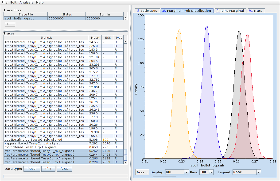
Each logged parameter is a sample from its own posterior distribution. Plot them, and summarise with a median and a 95% credible interval.
Tree samples
- Any question with a yes or no answer can be answered by counting: the posterior probability that a clade exists is the fraction of sampled trees containing it.
- Any quantity can be summarised the same way, for example the age of the common ancestor of two species, which has a full posterior distribution.
- Summary trees condense the sample into one picture. Common choices are the majority-rule consensus tree (clades in more than half of the sampled trees) and the maximum clade credibility tree, which BEAST produces with TreeAnnotator.
A summary tree is a summary, not the result. Branches with low posterior probability are drawn just as solidly as branches with high posterior probability, so always read the support values.
What a posterior probability on a branch means
A posterior probability of 0.93 on a branch means: given this alignment, this evolutionary model and these priors, there is a 93 percent chance that this grouping is real.
- This is a more direct statement than a bootstrap value, which describes how often the grouping recurs in resampled data rather than how probable it is.
- The qualification matters. The number is conditional on the model being adequate. If the model is wrong, a high posterior probability can be confidently wrong.
Software
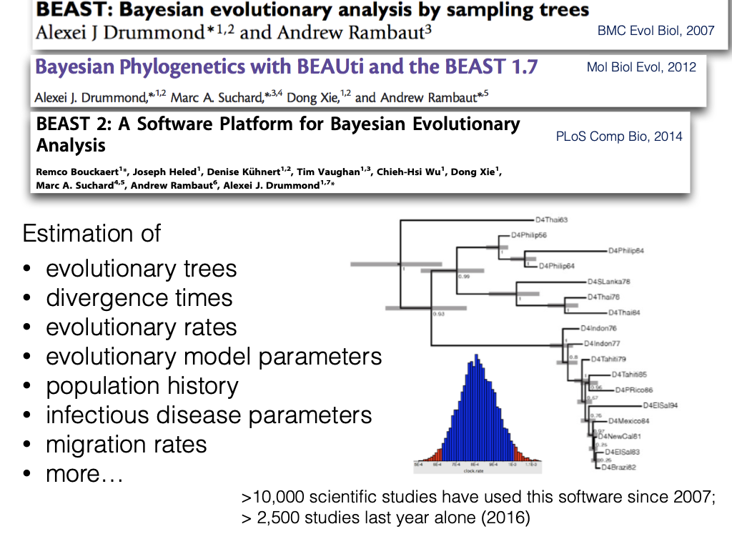
- BEAST 2 (Bouckaert et al., 2014)
- Dated trees, coalescent and birth-death tree priors, molecular clocks. This is what you will meet in the laboratory.
- MrBayes (Huelsenbeck and Ronquist, 2001)
- Long-established program for Bayesian phylogenetics.
- RevBayes (Höhna et al., 2016)
- Models are written out explicitly in a scripting language.
Summary
- Bayesian inference combines a prior with a likelihood to give a posterior distribution, which represents what we believe after seeing the data, uncertainty included.
- In phylogenetics the posterior covers the tree, the branch lengths and the model parameters together. It requires a tree prior, which is where the biology of speciation or of populations enters.
- There are far too many trees to enumerate, so we use MCMC: propose a small change, accept it if it improves the score, and accept it with probability equal to the score ratio if it does not.
- Only ratios of scores are needed, which is what makes the calculation possible at all.
- The output is a sample of trees. Posterior support for any feature is obtained by counting how often it appears.
- Convergence can be disproved but never proved. Run several chains, check ESS values, and be suspicious of a chain that looks too calm.
Recommended Reading
- Chapter 10: Bayesian inference, MCMC and Bayesian phylogenetics
Also useful:
- Nascimento, Reis & Yang (2017), "A biologist's guide to Bayesian phylogenetic analysis", Nature Ecology & Evolution 1:1446–1454.
- Drummond & Bouckaert (2015), Bayesian Evolutionary Analysis with BEAST.